This Is Not the ex-Gaussian Model You Are Looking For: On the Default Parameterization of Bayesian ex-Gaussian Models in brms

Jason Geller¹, Bernhard Angele², and Dominique Makowski³

¹Department of Psychology and Neuroscience, Boston College

²Nebrija University

³School of Psychology, University of Sussex

Author Note

Jason Geller Orcid ID Logo: A green circle with white letters ID https://orcid.org/0000-0002-7459-4505

Bernhard Angele Orcid ID Logo: A green circle with white letters ID https://orcid.org/0000-0001-8989-8555

Dominique Makowski Orcid ID Logo: A green circle with white letters ID https://orcid.org/0000-0001-5375-9967

The analyses herein were not preregistered. Data, code, and materials for this manuscript are available at https://github.com/jgeller112/exGauss_commentary. The entire manuscript, including all analyses and figures, can be reproduced by downloading the repository and following the instructions in its README. The authors have no conflicts of interest to disclose.

Author roles were classified using the Contributor Role Taxonomy (CRediT; https://credit.niso.org/) as follows: Jason Geller: conceptualization, data curation, formal analysis, project administration, resources, visualization, and writing – original draft. Bernhard Angele: formal analysis, validation, writing – original draft, and Writing - review & editing. Dominique Makowski: formal analysis, validation, software, and Writing - review & editing

Correspondence concerning this article should be addressed to Jason Geller, Department of Psychology and Neuroscience, Boston College, McGuinn 300, Chestnut Hill, MA 2467, USA, Email: drjasongeller@gmail.com

Abstract

The ex-Gaussian distribution is a popular mathematical model for analyzing response time (RT) data because it separates the central portion of the distribution, captured by the Gaussian parameters \mu and \sigma, from the positively skewed tail, captured by the exponential parameter \tau. Researchers often use these parameters to make inferences about underlying cognitive processes. As Bayesian methods have become increasingly accessible, complex ex-Gaussian models can now be fit with relative ease, and in R, the {brms} package makes this especially straightforward. However, it is important to recognize that the default parameterization offered by {brms} does not map onto the classical parameterization familiar to many researchers in experimental psychology in the default model, \mu indexes the mean of the full ex-Gaussian distribution rather than the location of the Gaussian component alone. This distinction matters because changes in the Gaussian location and changes in the exponential tail can offset one another at the level of the overall mean, so some published studies may have drawn incorrect inferences from effects estimated on the default \mu parameter. Using simulated data and a published finding we highlight how using the default parameterization can lead to misleading inferences. We then demonstrate how to fit the classical parameterization directly using the {cogmod} package, with the aim of helping researchers and reviewers align ex-Gaussian model parameters with their theoretical questions.

Keywords: ex-Gaussian, reaction time, Bayesian estimation, brms, parameterization

Word Count: 15144

Over the past two decades, psychology has seen a substantial rise in the application of Bayesian data analysis methods as a supplement to widely used frequentist methods (Pfadt et al., 2025). This shift has been driven by the increasing availability of computational tools that have made fitting Bayesian models both practical and efficient. Programming languages like R (R Core Team, 2026), Python (Van Rossum & Drake, 2009), and Julia (Bezanson et al., 2017) provide libraries and packages that allow researchers to fit Bayesian models with little technical overhead. In addition, growing dissatisfaction with the null ritual and its associated pitfalls (e.g., p-value misinterpretation and dichotomous thinking) (Gigerenzer, 2018), together with growing distrust of published findings, has pushed many researchers toward statistical alternatives (Vazire, 2018).

One domain that has seen increased adoption of Bayesian methods is experimental psychology, where one of the most common dependent variables is response times (RT), which is a measure of how long it takes a person to initiate a response (e.g., motor, written, or spoken) to a stimulus. RT data offers a window into cognitive processes underlying behavior (Baayen & Milin, 2010). Traditionally, RT data have been analyzed using summary statistics such as the mean or median. However, RT distributions are typically positively skewed, bounded at zero, and characterized by substantial variability both within and between individuals (Whelan, 2008; Wilcox & Keselman, 2003). Moreover, experimental manipulations may affect not only the central tendency of the distribution but also its variability or upper tail. Consequently, analyses based solely on the mean or median can obscure theoretically meaningful distributional effects, motivating calls to move beyond mean-based analyses of RT data (Balota & Yap, 2011).

One way to move beyond the mean is to model the full shape of the RT distribution. Mathematical models provide a flexible way to do so, allowing researchers to draw inferences about the psychological processes—such as memory, attention, and language—that give rise to observed response times. One model that has become especially popular for this purpose is the ex-Gaussian model (Ratcliff & Murdock, 1976). The ex-Gaussian distribution is formed by the convolution of a Gaussian distribution and an exponential distribution and is characterized by three parameters: \mu, \sigma, and \tau. The parameter \mu represents the mean of the Gaussian component, whereas \sigma represents its standard deviation. The \tau parameter represents both the mean and standard deviation of the exponential component and primarily governs the length of the distribution’s positively skewed upper tail. The overall mean of the ex-Gaussian distribution is \mu + \tau , and the standard deviation (SD) is \sqrt{\sigma^2+\tau^2} . Although these parameters have been used to infer cognitive processes such as automaticity (Balota et al., 2008; Dewitt et al., 2018) and cognitive control/inhibition (Kane & Engle, 2003), these interpretations are not inherent to the parameters and should be made cautiously (Matzke & Wagenmakers, 2009). Nevertheless, the ex-Gaussian model can provide a more complete description of RT data than the arithmetic mean alone, which can be disproportionately influenced by the positively skewed tail of the distribution.

The ex-Gaussian model can be fit within a Bayesian framework relatively easily using the {brms} package (Bürkner, 2017, 2018, 2021) in R, which provides a high-level interface to the probabilistic programming language Stan (Carpenter et al., 2017). The {brms} package supports a wide range of response distributions, including the ex-Gaussian family, and allows researchers to incorporate complex model structures at both the participant and item levels as well as across different parameters. This accessibility has contributed to the growing use of Bayesian ex-Gaussian models in reaction-time research (see Angele et al., 2023, 2024; Geller et al., 2025; Kinoshita & Liong, 2023; Serrano-Carot et al., 2026). However, an important complication arises from the default parameterization used by the R package {brms}. Although the model is straightforward to estimate, its default specification does not necessarily provide direct access to the parameter-specific comparisons researchers often wish to make.

The central problem is that the parameter labeled \mu in the default {brms} ex-Gaussian model does not correspond to the mean of the Gaussian component in the conventional parameterization. Instead, the quantity modeled as \mu in {brms} represents the mean of the full ex-Gaussian distribution. Under the conventional parameterization, this quantity is equal to \mu_{\mathrm{Gaussian}} + \tau. Consequently, regression effects estimated for the default \mu parameter reflect changes in a composite quantity that combines the Gaussian location and exponential tail components. Such effects therefore cannot be interpreted directly as changes in the Gaussian component or in typical response speed. To recover the conventional Gaussian mean, it is necessary to derive it from the model parameters as \mu_{\mathrm{Gaussian}} = \mu_{\mathrm{brms}} - \tau or to specify an alternative parameterization that models the conventional ex-Gaussian parameters directly.

In this paper, we demonstrate what the default parameterization of the ex-Gaussian model in {brms} actually represents, and then show how to reparameterize the model so that \mu corresponds to the location of the Gaussian component — the conventional ex-Gaussian parameter used in RT research — rather than the mean of the full distribution. We illustrate this first with a simulated dataset and then through reanalysis of a published finding. Our goal is to improve the accuracy and interpretability of inferences drawn from these models. This issue is particularly important because the ex-Gaussian distribution is widely used to distinguish changes in the central portion of the RT distribution from changes in its positively skewed tail.

Simulation Example

Data Generation

To demonstrate the issue with fitting the default ex-Gaussian model in {brms}, we simulate data using a comparison adapted from one of our own studies (Geller et al., 2025) in R (version 4.6.1, R Core Team, 2026)¹. In Geller et al. (2025), we examined how perceptual disfluency—manipulated by varying the level of blur applied to letter strings influenced reaction times in a lexical decision task (LDT; i.e., is this letter string a word?), and whether these effects were related to how well someone remembers the words in a recognition memory task. In that study, low blur words affected early stages of encoding, reflected in the Gaussian location parameter \mu, but not the later, tail component captured by \tau. For the present illustration, however, we construct a sharper scenario in which \mu and \tau differ in opposite directions so that the two conditions share the same expected reaction time. Using the classical ex-Gaussian parameterization implemented in the {cogmod} package (Makowski, 2026), we simulate ex-Gaussian data for clearly presented and low-blur words in which \mu is set to 500 ms and 550 ms, \tau to 100 ms and 50 ms, and \sigma to 60 ms in both conditions (see Table 1).

Listing 1: Installing and loading the {cogmod} package from GitHub.

Show R code

# install from Github
#remotes::install_github("DominiqueMakowski/cogmod")

library(cogmod)

Table 1

Data-generating ex-Gaussian parameters for the Clear and Low-Blur conditions, with opposing changes in \mu and \tau that hold the expected response time (\mu+\tau) constant.

Blur	μ	σ	τ	Expected RT
Clear	500	60	100	600
Low-Blur	550	60	50	600

To simulate the data, We first draw 100 reaction times per condition (200 in total) from the ex-Gaussian distributions defined by these parameters (Listing 2).

Listing 2: Simulating ex-Gaussian reaction times for the Clear and Low-Blur conditions.

Show R code

# Fix the random seed so the simulated data are identical on every render.
set.seed(1234)

# Number of simulated trials per condition (200 observations in total).
n_per_group <- 100

# One row per trial, labelled by Blur condition (Clear is the reference level).
d <- data.frame(
  Blur = factor(
    rep(c("Clear", "Low-Blur"), each = n_per_group),
    levels = c("Clear", "Low-Blur")
  )
)

# Row index (1 = Clear, 2 = Low-Blur) used to look up each trial's parameters.
parameter_index <- as.integer(d$Blur)

# Draw reaction times from the classical ex-Gaussian using each trial's
# condition values, via {cogmod}'s rrt_exgaussian() generator.
d$rt <- cogmod::rrt_exgaussian(
  n = nrow(d),
  mu = sim_params$mu[parameter_index],
  sigma = sim_params$sigma[parameter_index],
  tau = sim_params$tau[parameter_index]
)

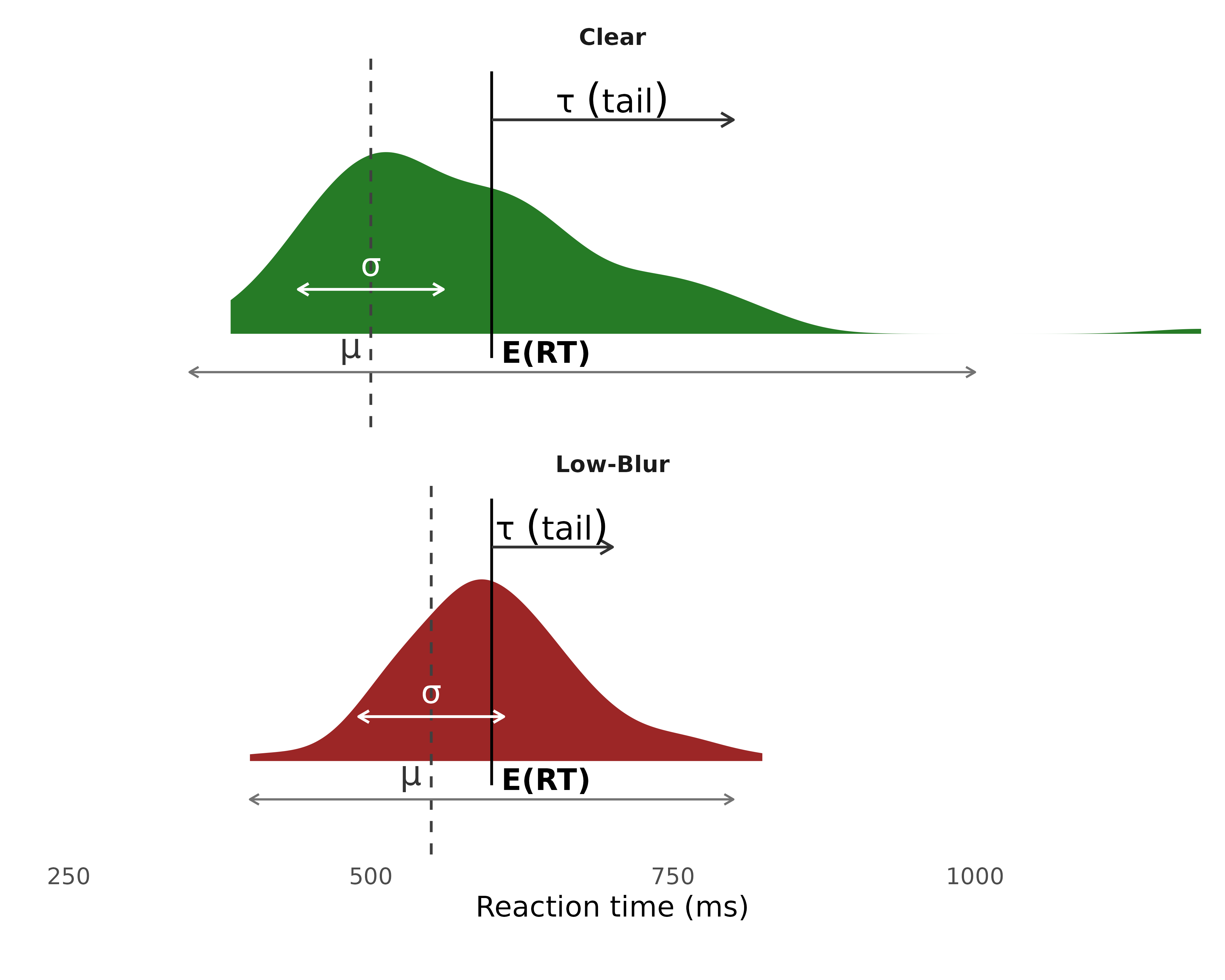
Figure 1 shows the simulated RT distribution for each condition and how the three ex-Gaussian parameters shape it: \mu locates the Gaussian component, \sigma sets its spread, and \tau stretches the right tail. Because the increase in \mu from Clear to Low-Blur is offset by an equal decrease in \tau, the overall mean E(RT) = \mu + \tau is identical (600 ms) in both conditions.

Figure 1

Simulated reaction-time distributions for each condition, annotated with the ex-Gaussian parameters. The dashed line marks the Gaussian location \mu; the double arrow spans \pm\sigma around it (the Gaussian spread); the rightward arrow over the tail marks the exponential component \tau, which stretches the distribution to the right; and the solid line marks the overall mean E(RT) = \mu + \tau, which is 600 ms in both conditions. The bottom span highlights that E(RT) is the mean of the *entire* distribution — the quantity the default `brms` `mu` estimates.

Default {brms} Parameterization

Using this data we fit the default brms ex-Gaussian model. In this parameterization, the parameter labeled mu represents the expected value of the full ex-Gaussian distribution rather than the location of its Gaussian component.

The exponential component is labeled beta. On the response scale, beta corresponds to the classical ex-Gaussian parameter \tau:

\beta_{\texttt{brms}} = \tau_{\text{classical}}.

Thus, beta and \tau are not substantively different quantities. Both represent the mean of the exponential component. The difference is primarily one of notation. The important difference between the default {brms} model and the classical parameterization concerns mu:

\mu_{\texttt{brms}} = \mu_{\text{classical}} + \tau.

In other words, the default {brms} parameterization uses mu for the expected value of the complete ex-Gaussian distribution, whereas the classical parameterization uses \mu for the location of the Gaussian component.

Both the expected response and the exponential component are allowed to vary across conditions.

Prior Specification

The priors were selected to reflect the known scale of the simulated data while remaining sufficiently broad to allow the model to recover deviations from the generating values. Table 2 shows these priors alongside those used for the classical parameterization introduced later, so the two specifications can be compared directly.

Table 2

Prior specification for the default and classical ex-Gaussian models.

Parameter	Default Prior	Classical Prior	Notes
Intercept (μ)	Normal(600, 100)	Normal(500, 100)	Same form; centered on each parameterization's reference-condition value (E(RT) = 600 ms vs. Gaussian location = 500 ms); both mu and E(RT) use an identity link, so both priors are on the response scale
Blur (μ)	Normal(0, 50)	Normal(0, 50)	Identical across parameterizations; no assumed direction for the effect of Blur
Intercept (β / τ)	Normal(log(100), 0.5)	Normal(log(100), 0.5)	Identical form in both models: brms's native `exgaussian()` and {cogmod}'s `rt_exgaussian()` (here fit with `link_tau = "log"`) both use a log link for the exponential component, so the prior is on the log scale, centered at log(100 ms)
Blur (β / τ)	Normal(0, 0.5)	Normal(0, 0.5)	Identical across parameterizations; no assumed direction for the effect of Blur, expressed on the log scale
Intercept (σ)	brms default	Normal(log(60), 0.5)	Only the classical model estimates sigma explicitly; fit with `link_sigma = "log"`, so the prior is on the log scale, centered at log(60 ms)

In {brms}, the bf() function combines separate linear-model formulas for each parameter of the response distribution into a single distributional-formula object passed to brm(). For the ex-Gaussian family, this lets mu, sigma, and beta each be modeled by their own predictors within one call: below, rt ~ Blur models mu as a function of Blur, sigma ~ 1 holds the Gaussian standard deviation constant across conditions, and beta ~ Blur allows the exponential mean to vary by Blur as well. The model is fit with 2 MCMC chains of 2,000 iterations each (including 500 warmup iterations), more than sufficient for a model this simple.

The model can then be fit as follows (Listing 3):

Listing 3: Fitting the default ex-Gaussian model in brms.

Show R code

fit_brms <- brm(
  bf(
    rt ~ Blur, # mu submodel: here mu is E(RT), not the Gaussian location
    sigma ~ 1, # constant Gaussian SD
    beta ~ Blur # exponential mean (the classical tau), allowed to vary
  ),
  data = d,
  prior = priors_default, # priors from above
  family = exgaussian(), # brms' built-in ex-Gaussian family
  chains = 2,
  iter = 2000, 
  warmup = 500,
  backend = "cmdstanr",
  cores = 4,
  seed = 1234, # reproducible draws
  file = file.path(fits_dir, "fit-default"), # cache: skip refitting if unchanged
  file_refit = "on_change" # but do refit if the model spec above changes
)

Estimating Ex-Gaussian Parameters

The {modelbased} package (Makowski et al., 2025), which is part of the {easystats} ecosystem (Lüdecke et al., 2019), can easily be used to obtain condition-specific posterior estimates from a fitted model. The estimate_means() function returns estimated parameters for each condition, back-transformed, so estimates are presented on the scale of interest (here milliseconds), whereas estimate_contrasts() computes differences between conditions. To conserve space this code is not shown here, but interested readers can go to the GitHub repo and view the code.

Throughout this paper, we treat an effect as reflecting a credible difference when its 95% credible interval excludes zero and its probability of direction (pd) [i.e., the probability that the posterior distribution is strictly positive or negative) (Makowski et al., 2025) exceeds ~97%. When either condition fails to hold, we describe the effect as non-credible or uncertain.

As shown in Table 1, the present data were generated so that the two conditions have the same expected reaction time but differ in the Gaussian and exponential components of the ex-Gaussian distribution.

Under the classical ex-Gaussian parameterization, the expected response is

E(RT) = \mu + \tau.

Thus, the 50-ms increase in \mu for the Low-Blur condition is offset by a 50-ms decrease in \tau. The expected RT is therefore 600 ms in both conditions.

Estimating the Expected Response (\mu)

Condition-specific estimates of the expected response can be obtained with estimate_means() and setting predict argument to “mu”.

Because the primary mu parameter in the default ex-Gaussian model represents E(RT), these estimates should be close to 600 ms in both conditions.

The corresponding contrast can be obtained using estimate_contrasts() (see Table 4).

The posterior estimate of this contrast should be close to zero because the two conditions were generated with the same expected RT:

(550 + 50) - (500 + 100) = 600 - 600 = 0.

Estimating the Exponential Component

In the default {brms} parameterization, beta represents the mean of the exponential component. It therefore corresponds directly to \tau in the classical parameterization:

\beta = \tau.

Condition-specific estimates can be obtained by requesting predictions for beta.

Although the resulting object is called tau_estimates_default for interpretive clarity, the parameter is named beta inside the default brm model. Table 3 shows both the expected response and the exponential component together, by condition.

Table 3

Estimated expected response, E(RT), and exponential component (beta), by condition from the default brms model.

Blur	Parameter	Mean [95% CrI]
Clear	E(RT)	581.4 [559.8, 606.3]
	β	108.1 [79.9, 140.2]
Low-Blur	E(RT)	603.4 [588.5, 619.7]
	β	56.4 [35.3, 80.0]

These estimates should be close to 600 ms for E(RT) in both conditions, and approximately 100 ms for Clear and 50 ms for Low-Blur for beta.

The corresponding contrasts can be obtained using estimate_contrasts() (see Table 4).

Table 4

Blur contrast in the expected response, E(RT), and the exponential component (beta), from the default brms model.

Contrast	Parameter	Mean [95% CrI]	pd
Low-Blur - Clear	E(RT)	22.0 [-5.4, 48.8]	0.943
Low-Blur - Clear	β	-51.7 [-87.1, -19.6]	1.000

As shown in Table 4, the default model correctly recovers a near-zero contrast in E(RT), since the two conditions were generated with the same expected RT. However, its primary mu coefficient does not directly reveal the 50-ms difference in the Gaussian-location parameter — that difference only shows up in the beta contrast, which is approximately 50 ms.

Classical Ex-Gaussian Parameterization

As we have shown above, the default parameterization yields the expected RT of the entire distribution. We can instead fit the model using the rt_exgaussian() family from the {cogmod} package, which implements the classical ex-Gaussian parameterization. In this model, \mu represents the location of the Gaussian component and \tau represents the mean of the exponential component.

By default, {cogmod} links all three parameters with a softplus function, rather than the identity or log links {brms} typically applies. An identity link would let the linear predictor cross zero, which is invalid for all three parameters, since \mu must stay positive to represent a genuine RT-scale location, and \sigma and \tau are positive by definition. Softplus keeps the positivity constraint but behaves almost linearly away from zero, which is convenient in principle — but only in the positive direction, and only once the linear predictor is comfortably greater than zero: \text{softplus}(x) = \log(1+e^x) \to x as x \to \infty, but \text{softplus}(x) \to 0 as x \to -\infty, so the link is sharply nonlinear for negative or near-zero linear predictors (e.g., \text{softplus}(-2) \approx 0.13, nothing like -2). Whether a response-scale prior actually lands in that near-linear region depends on the measurement scale of the outcome, not just the link function itself — the same nominal prior can behave very differently depending on whether an RT is coded in milliseconds or seconds.

Because of this scale-sensitivity, and because we would rather interpret every coefficient directly in estimate_means()/estimate_contrasts() output than reason about a link function at all, we do not use {cogmod}’s default softplus link in this paper. rt_exgaussian() accepts link_mu, link_sigma, and link_tau arguments so each parameter’s link can be set independently; we use an identity link for \mu and a log link for \sigma and \tau — the same links {brms}’s own built-in exgaussian() family uses for its location and scale parameters, and a familiar, scale-robust choice for enforcing positivity (unlike softplus, log’s behavior does not depend on whether the parameter values happen to be small or large in absolute terms). The model is specified with family = rt_exgaussian(link = "identity", link_sigma = "log", link_tau = "log").

At the sampling level, the log-likelihood is written in Stan and calls the built-in exp_mod_normal_lpdf() function², which implements the exponentially modified Gaussian density. That built-in function is parameterized by the rate of the exponential component rather than its mean, so \tau is converted internally via 1/\tau before being passed in. The custom family simply relabels and re-links Stan’s existing exponentially modified Gaussian implementation.

Prior Specification

The priors for the classical model follow the same reasoning as those for the default model, shown together in Table 2:

As before, bf() combines the per-parameter formulas into a single distributional model, but now mu is the Gaussian location itself, tau (rather than beta) carries the exponential-mean submodel, and sigma is estimated explicitly via its own formula rather than left to a family default. The model is then fit using (Listing 4):

Listing 4: Fitting the classical ex-Gaussian model using {cogmod}.

Show R code

fit_brms_new <- brm(
  bf(
    rt ~ Blur, # mu submodel: here mu IS the Gaussian location
    tau ~ Blur, # exponential mean (the tail), allowed to vary
    sigma ~ 1 # constant Gaussian SD
  ),
  data = d,
  prior = priors_classical,
  family = rt_exgaussian(
    link = "identity",
    link_sigma = "log",
    link_tau = "log"
  ), # {cogmod} family with identity/log links
  stanvars = rt_exgaussian_stanvars(), # Stan code injected into the model
  chains = 2,
  iter = 2000,
  warmup = 500,
  backend = "cmdstanr",
  cores = 4,
  seed = 1234,
  file = file.path(fits_dir, "fit-classical"), # cache: skip refitting if unchanged
  file_refit = "on_change" # but do refit if the model spec above changes
)

Estimating the Gaussian-Location Parameter

For the classical model, estimates from the primary regression formula correspond to the Gaussian-location parameter \mu.

The estimates are approximately 500 ms for Clear and 550 ms for Low-Blur.

The contrast between the two can be obtained using estimate_contrasts() (see Table 6).

The posterior mean will not necessarily equal exactly 50 ms because of sampling variability. However, the 95% credible interval should contain the population value of 50 ms when the model successfully recovers the simulated effect.

Estimating the Exponential Component

Condition-specific estimates of \tau can be obtained by requesting predictions for the tau distributional parameter.

Table 5 shows the Gaussian-location and exponential-component estimates together, by condition.

Table 5

Estimated Gaussian-location (\mu) and exponential (\tau) parameters, by condition, from the classical model.

Blur	Parameter	Mean [95% CrI]
Clear	μ	477.1 [453.6, 503.0]
	τ	103.8 [75.9, 134.0]
Low-Blur	μ	545.1 [523.9, 566.0]
	τ	57.8 [36.5, 81.1]

The estimates should be close to 100 ms for Clear and 50 ms for Low-Blur for \tau.

The corresponding contrast can be obtained using estimate_contrasts() (see Table 6).

Table 6

Blur contrast in the Gaussian-location (\mu) and exponential (\tau) parameters, from the classical model.

Contrast	Parameter	Mean [95% CrI]	pd
Low-Blur - Clear	μ	68.0 [40.4, 95.2]	1.000
Low-Blur - Clear	τ	-46.0 [-78.3, -15.3]	0.998

The results seen in Table 6 are very similar to those from the default parameterization for \tau, but unlike the default model, the classical model’s \mu contrast directly recovers the simulated 50-ms shift in the Gaussian location.

This example illustrates the central difference between the two parameterizations. The default {brms} ex-Gaussian model directly estimates the expected response and labels that parameter mu. The exponential component is labeled beta, although it corresponds to the classical \tau parameter. In contrast, the {cogmod}’s rt_exgaussian() model uses mu for the Gaussian-location parameter and tau for the exponential mean, consistent with the classical parameterization commonly used in reaction-time research.

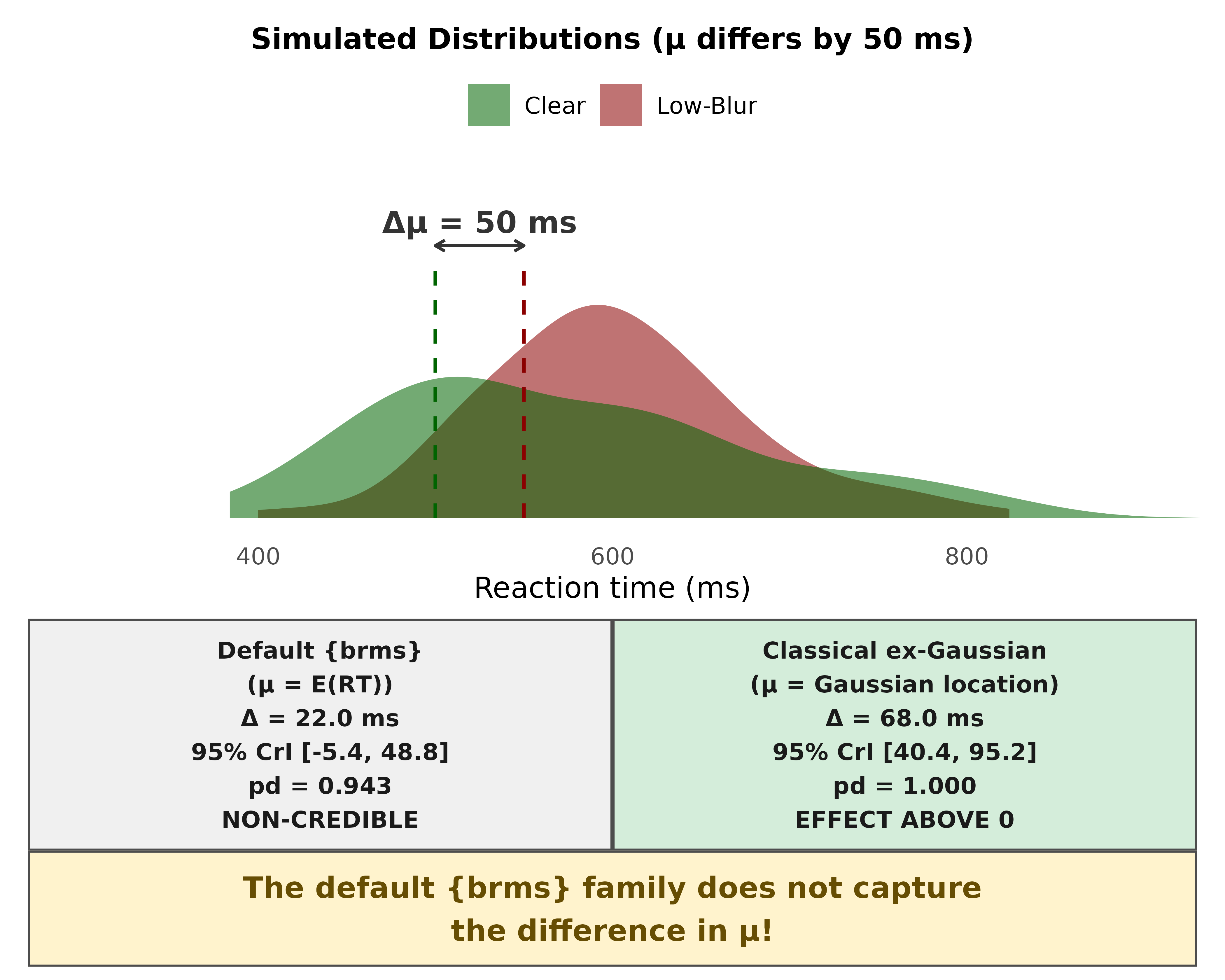
Figure 2 summarizes this simulation in a single picture: the two simulated distributions differ by 50 ms in the Gaussian location \mu, but only the classical parameterization’s contrast on \mu detects that difference — the default {brms} model’s contrast (on E(RT)) does not.

Figure 2

Graphical summary of the Simulation Example. Top: simulated reaction-time distributions for the Clear and Low-Blur conditions, which differ by 50 ms in the Gaussian location \mu. Bottom: the Blur contrast under each parameterization, with credibility determined by whether the 95% credible interval excludes zero; pd is the probability of direction.

From Simulation to Application: Reanalysis of Angele et al. (2023)

In order to demonstrate how the difference between parameterizations can affect the interpretation of real data, we re-analyze Experiment 1 from Angele et al. (2023). The main focus of Angele et al. (2023)’s study was to test whether the masked priming paradigm can be successfully implemented in a JavaScript-based online experiment built in PsychoPy (Peirce et al., 2019) and hosted on Pavlovia. In a prototypical masked priming task (Forster & Davis, 1984), a stimulus (called the prime) is presented for a very short duration and immediately replaced by a target stimulus in the same location in upper case, on which participants must judge lexicality. Angele et al. (2023) used masked identity priming, in which the prime is either identical to the target (e.g., region–REGION) or unrelated (e.g., launch–REGION). While testing whether masked priming could be obtained in an online setting was one goal, Angele et al. (2023) also attempted to make a theoretical contribution by using the ex-Gaussian model to evaluate Forster (1998)’s savings hypothesis. Forster (1998) argued that if the prime is identical to the target, having pre-processed the prime will allow participants to respond faster. In this case, the whole distribution of reaction times should be shifted to the left for the identical condition compared to the unrelated condition — that is, there should be an effect on \mu rather than on the slower responses (i.e., \tau). The experiment had a 2 × 2 design, crossing prime exposure duration (33.3 ms vs. 50 ms) with priming condition (Identical vs. Unrelated). Consistent with the savings hypothesis, they found a robust effect of relatedness on \mu, with responses to the unrelated condition being slower on average than to the identical condition, and this priming effect was larger at the 50-ms exposure duration than at 33.3 ms (see Table 9 for estimates from this experiment). Critically, relatedness had no credible effect on \tau, indicating that the priming manipulation shifted the RT distribution rather than changing its shape.

To fit their ex-Gaussian models, Angele et al. (2023) used the built-in exgaussian() family in {brms}. As established above, the primary formula in default {brms} models the overall distributional mean E(RT) = \mu_{\text{Gaussian}} + \tau, despite assigning the label mu to this parameter. In their manuscript, Angele et al. (2023) interpreted regression effects on mu as changes in the location of the Gaussian component \mu.

Here, we apply the classical ex-Gaussian parameterization using {cogmod}, modeling reaction times with maximal random intercepts and random slopes for participants (source) and items (Target) across both \mu (Gaussian location) and \tau (exponential mean). Reaction time is coded in milliseconds in this dataset. As discussed above, we fit this model with link_mu = "identity" and link_sigma = link_tau = "log" rather than {cogmod}’s default softplus links, so priors and raw model coefficients for \mu are directly on the millisecond scale, and priors for \sigma and \tau are on the (familiar, scale-robust) log scale. As with the simulated example, all condition-specific estimates and contrasts are still obtained through estimate_means()/estimate_contrasts() rather than by reading the raw coefficients directly.

Prior specification for the classical model is summarized in Table 7.

Table 7

Prior specification for the classical ex-Gaussian model fit to Experiment 1 from Angele et al. (2023).

Parameter	Prior
Intercept (μ)	Normal(500, 100)
Condition (μ)	Normal(0, 100)
Prime Duration (μ)	Normal(0, 100)
Condition x Prime Duration (μ)	Normal(0, 100)
Intercept (τ)	Normal(log(100), 0.5)
All effects (τ)	Normal(0, 0.5)
Intercept (σ)	Normal(log(60), 0.5)

The classical ex-Gaussian model for Experiment 1 is specified and fit as follows (Listing 5):

Listing 5: Fitting the classical ex-Gaussian hierarchical model to Experiment 1 from Angele et al. (2023).

Show R code

# Fit classical ex-Gaussian hierarchical model to Experiment 1 RT data
blmm_exp1_classical_rt <- brm(
  data = data_fit,
  formula = bf(
    rt ~ Condition *
      PrimeDuration +
      (1 + Condition * PrimeDuration | source) +
      (1 + Condition * PrimeDuration | Target),
    tau ~ Condition *
      PrimeDuration +
      (1 + Condition * PrimeDuration | source) +
      (1 + Condition * PrimeDuration | Target),
    sigma ~ 1
  ),
  warmup = 1000,
  iter = 5000,
  chains = 4,
  prior = priors_classical,
  family = rt_exgaussian(
    link = "identity",
    link_tau = "log",
    link_sigma = "log"
  ), # {cogmod} family with identity/log links
  stanvars = rt_exgaussian_stanvars(), # Stan code injected into the model
  init = 0,
  cores = 4,
  backend = "cmdstanr",
  threads = threading(2)
)

Depending on the hardware used, this model may take more than 30 minutes to fit. Because of this, it is recommended to fit it once and then save the fitted model object to a file for later use.

Estimating Ex-Gaussian Parameters with `{easystats}`

As in the Simulation Example, we use {modelbased}’s estimate_means() and estimate_contrasts() to obtain condition-specific posterior estimates and contrasts, rather than computing them by hand from the raw posterior draws. Because this model has thousands of posterior draws and a large number of by-participant and by-item random effects, we set backend = "emmeans" (instead of the default marginaleffects backend) to keep the marginal computations memory-efficient.

Table 8

Estimated Gaussian-location (\mu) and exponential (\tau) parameters by condition and prime duration for Experiment 1 from Angele et al. (2023) under the classical model.

Condition	PrimeDuration	Parameter	Mean [95% CrI]
Identical	33 ms	μ	509.9 [494.7, 525.8]
		τ	111.5 [101.5, 122.0]
	50 ms	μ	498.2 [482.9, 514.4]
		τ	101.2 [90.8, 112.0]
Unrelated	33 ms	μ	529.8 [514.7, 545.6]
		τ	113.4 [102.5, 124.8]
	50 ms	μ	535.3 [520.3, 551.0]
		τ	105.3 [95.0, 116.0]

Table 8 displays the estimated posterior means for \mu and \tau across priming conditions and exposure durations. Table 9 below presents the model’s population-level effects (main effect of relatedness, main effect of prime duration, and their interaction) alongside simple priming contrasts (Unrelated minus Identical) at each prime duration, for both parameters side by side.

Table 9

Fixed effects and priming contrasts in the Gaussian-location (\mu) and exponential (\tau) parameters for Experiment 1 from Angele et al. (2023) under the classical model, alongside the default-brms E(RT) effects as originally reported by Angele et al. (2023). All estimates are in milliseconds and reflect Unrelated minus Identical (or 50 ms minus 33 ms) differences; pd is the probability of direction.

Effect	Default brms E(RT)	Parameter	Mean [95% CrI]	pd
Main Effect of Relatedness	31.5 [27.7, 35.3]	μ	-28.5 [-32.3, -24.7]	1.000
Main Effect of Relatedness		τ	-3.1 [-8.0, 1.9]	0.889
Main Effect of Duration	-10.9 [-14.5, -7.3]	μ	3.1 [-0.2, 6.4]	0.969
Main Effect of Duration		τ	9.2 [3.7, 14.8]	0.999
Relatedness × Duration	19.3 [12.6, 26.0]	μ	17.1 [10.5, 23.8]	1.000
Relatedness × Duration		τ	2.2 [-8.4, 12.6]	0.658
Priming Effect at 33 ms	~22.0	μ	-20.0 [-25.0, -15.0]	1.000
Priming Effect at 33 ms		τ	-1.9 [-9.3, 5.3]	0.699
Priming Effect at 50 ms	~41.0	μ	-37.1 [-42.1, -31.9]	1.000
Priming Effect at 50 ms		τ	-4.1 [-11.2, 3.2]	0.865

As shown in Table 9, under the classical parameterization, the true Gaussian location \mu shows a robust overall main effect of relatedness (-28.5 ms, 95% CrI [-32.3, -24.7], pd = 1.000). Unlike the effect reported as \mu under the default parameterization, the main effect of prime duration on \mu is non-credible under the classical parameterization (3.1 ms, 95% CrI [-0.2, 6.4], pd = 0.969, with the 95% CrI narrowly containing zero). The model also reveals a credible interaction between relatedness and prime duration (17.1 ms, 95% CrI [10.5, 23.8], pd = 1.000), indicating that the priming effect on \mu was larger at 50 ms (-37.1 ms, 95% CrI [-42.1, -31.9], pd = 1.000) than at 33 ms (-20.0 ms, 95% CrI [-25.0, -15.0], pd = 1.000).

For the exponential component \tau, the main effect of relatedness is small and non-credible (-3.1 ms, 95% CrI [-8.0, 1.9], pd = 0.889), as is the interaction term (2.2 ms, 95% CrI [-8.4, 12.6], pd = 0.658). Consequently, the priming effect (i.e., the difference between related and unrelated prime conditions) on \tau is non-credible at 33 ms (-1.9 ms, 95% CrI [-9.3, 5.3], pd = 0.699) and 50 ms (-4.1 ms, 95% CrI [-11.2, 3.2], pd = 0.865), consistent with Forster’s (1998) savings hypothesis that would expect such an effect to show in \mu rather than in \tau. However, the model reveals a credible main effect of prime duration on \tau (9.2 ms, 95% CrI [3.7, 14.8], pd = 0.999), showing that increasing prime duration from 33 ms to 50 ms moderately shortened the right tail.

Comparison with Angele et al. (2023)

Comparing these classical ex-Gaussian estimates with those originally reported by Angele et al. (2023) (the “Default brms E(RT)” column of Table 9) highlights the practical consequences of model parameterization for theoretical inferences.

Parameter Interpretation. Angele et al. (2023) reported fixed effects for relatedness, prime duration, and their interaction from default {brms} under the assumption that mu represented the Gaussian location component \mu_{\text{Gaussian}}. Actually, the brms default mu estimates E(RT) = \mu_{\text{Gaussian}} + \tau. Consequently, Angele et al. (2023) interpreted overall differences in the distribution mean E(RT) as changes in the Gaussian location \mu_{\text{Gaussian}}, when in fact they were a composite of changes in both \mu_{\text{Gaussian}} and \tau.
Prime Duration Effects: While Angele et al. (2023)’s interpretation of most of the effects does not differ substantially from what the classical parameterization results indicate, there is one interesting and potentially theoretically relevant difference: Based on their default {brms} model, Angele et al. (2023) concluded that increasing prime exposure duration from 33 ms to 50 ms produced a credible downward shift in the Gaussian location parameter \mu (b = -10.9 ms, 95% CrI [-14.5, -7.3]). However, the classical parameterization reveals that the true main effect of prime duration on \mu_{\text{Gaussian}} is uncertain (3.1 ms, 95% CrI [-0.2, 6.4], pd = 0.969, with the 95% CrI containing zero). Instead, our reanalysis shows that the overall reduction in RTs at 50 ms prime duration was driven almost entirely by a compression of the exponential tail \tau (9.2 ms, 95% CrI [3.7, 14.8], pd = 0.999). The effect on E(RT) reported by Angele et al. (2023) as a location shift in \mu was actually the composite sum of a non-credible \mu shift (3.1 ms) and a credible \tau tail reduction (9.2 ms).
Priming Effects and Interaction: For the priming manipulation, the main effect of relatedness on \mu_{\text{Gaussian}} (-28.5 ms, 95% CrI [-32.3, -24.7], pd = 1.000) and the interaction (17.1 ms, 95% CrI [10.5, 23.8], pd = 1.000) closely mirror the E(RT) effects reported by Angele et al. (2023) (main effect \sim 31.5 ms, interaction \sim 19.3 ms). The estimates for the two parameterizations align closely for the priming effect because \tau showed no credible priming differences (-3.1 ms, 95% CrI [-8.0, 1.9], pd = 0.889). When \Delta \tau \approx 0, changes in the distributional mean \Delta E(RT) track changes in the Gaussian location \Delta \mu nearly 1-to-1.
Summary: This empirical comparison demonstrates that misinterpreting default {brms} parameters can lead to subtle misattributions regarding which distributional component is altered by an experimental manipulation. In Angele et al. (2023), a tail-shortening effect of prime duration (\Delta \tau = 9.2 ms) was attributed to the Gaussian location parameter (mu). Adopting the classical parameterization showcases some uncertainty regarding the existence of an effect of prime duration on \mu (pd = 0.969), underscoring that parameterization affects not only which component an effect is attributed to, but the confidence with which its existence can be claimed at all.

Conclusion

With this discussion, we hope to encourage researchers to use the appropriate ex-Gaussian parameterization when modeling reaction-time data with the {brms} package. The ex-Gaussian distribution provides a powerful framework for moving beyond analyses of the mean by separating differences in the central portion of the reaction-time distribution from differences in its right tail.

However, this flexibility also requires careful attention to model parameterization. In particular, researchers should not assume that parameters with familiar labels necessarily have the same interpretation across software implementations. Researchers should therefore examine the statistical definition and underlying implementation of a model before fitting it and interpreting its parameters. This is especially important when using flexible modeling software that may adopt parameterizations that differ from those commonly used in a particular research literature. We hope this commentary serves both as a practical guide to fitting the classical ex-Gaussian model in {brms} and as a broader reminder that convenient software defaults should not replace careful consideration of what a model actually estimates.

Declarations

Funding

No funding to report.

Conflicts of Interest

The authors declare no conflicts of interest.

Ethics Approval

Not applicable. No human data was collected.

Availability of Data, Code, and Materials

All data and code are stored here: https://github.com/jgeller112/exGauss_commentary.

Authors’ Contributions

JG - Conceptualization, Data curation, Formal analysis, Project administration, Resources, Visualization, Writing—original draft
BA - Formal analysis, Validation, Writing—original draft, Writing—review & editing
DM - Formal analysis, Validation, Software, Writing—review & editing

References

Allaire, J., Xie, Y., Dervieux, C., McPherson, J., Luraschi, J., Ushey, K., Atkins, A., Wickham, H., Cheng, J., Chang, W., & Iannone, R. (2026). rmarkdown: Dynamic documents for r. https://github.com/rstudio/rmarkdown

Angele, B., Baciero, A., Gómez, P., & Perea, M. (2023). Does online masked priming pass the test? The effects of prime exposure duration on masked identity priming. Behavior Research Methods, 55(1), 151–167. https://doi.org/10.3758/s13428-021-01742-y

Angele, B., Gutiérrez-Cordero, I., Perea, M., & Marcet, A. (2024). Reading(,) with and without commas. Quarterly Journal of Experimental Psychology, 77(6), 1190–1200. https://doi.org/10.1177/17470218231200338

Arel-Bundock, V. (2026). tinytable: Simple and configurable tables in “HTML,” “LaTeX,” “Markdown,” “Word,” “PNG,” “PDF,” and “Typst” formats. https://doi.org/10.32614/CRAN.package.tinytable

Baayen, R. H., & Milin, P. (2010). Analyzing reaction times. International Journal of Psychological Research, 3(2), 12–28. https://doi.org/10.21500/20112084.807

Balota, D. A., & Yap, M. J. (2011). Moving beyond the mean in studies of mental chronometry the power of response time distributional analyses. Current Directions in Psychological Science, 20(3), 160166. https://doi.org/10.1177/0963721411408885

Balota, D. A., Yap, M. J., Cortese, M. J., & Watson, J. M. (2008). Beyond mean response latency: Response time distributional analyses of semantic priming and word frequency effects. Journal of Memory and Language, 59(4), 495–523. https://doi.org/10.1016/j.jml.2007.10.004

Bezanson, J., Edelman, A., Karpinski, S., & Shah, V. B. (2017). Julia: A fresh approach to numerical computing. SIAM Review, 59(1), 65–98. https://doi.org/10.1137/141000671

Bürkner, P.-C. (2017). brms: An R package for Bayesian multilevel models using Stan. Journal of Statistical Software, 80(1), 1–28. https://doi.org/10.18637/jss.v080.i01

Bürkner, P.-C. (2018). Advanced Bayesian multilevel modeling with the R package brms. The R Journal, 10(1), 395–411. https://doi.org/10.32614/RJ-2018-017

Bürkner, P.-C. (2021). Bayesian item response modeling in R with brms and Stan. Journal of Statistical Software, 100(5), 1–54. https://doi.org/10.18637/jss.v100.i05

Carpenter, B., Gelman, A., Hoffman, M. D., Lee, D., Goodrich, B., Betancourt, M., Brubaker, M. A., Guo, J., Li, P., & Riddell, A. (2017). Stan: A probabilistic programming language. Journal of Statistical Software, 76(1), 1–32. https://doi.org/10.18637/jss.v076.i01

Ching, T. (2026). qs2: Efficient serialization of r objects. https://doi.org/10.32614/CRAN.package.qs2

Dewitt, S. H., Lagnado, D., & Fenton, N. (2018). Updating prior beliefs based on ambiguous evidence (,. M. R. J. Z. Chuck Kalish & T. Rogers, Eds.; p. 306311).

Forster, K. I. (1998). The pros and cons of masked priming. Journal of Psycholinguistic Research, 27(2), 203–233. https://doi.org/10.1023/A:1023202116609

Forster, K. I., & Davis, C. (1984). Repetition priming and frequency attenuation in lexical access. Journal of Experimental Psychology: Learning, Memory, and Cognition, 10(4), 680–698. https://doi.org/10.1037/0278-7393.10.4.680

Geller, J., Gómez, P., Buchanan, E. M., & Makowski, D. (2025). A distributional response time analysis of the perceptual disfluency effect. Journal of Cognition, 8(1), 50. https://doi.org/10.5334/joc.469

Gigerenzer, G. (2018). Statistical rituals: The replication delusion and how we got there. Advances in Methods and Practices in Psychological Science, 1(2), 198–218. https://doi.org/10.1177/2515245918771329

Hester, J., Wickham, H., & Csárdi, G. (2026). fs: Cross-platform file system operations based on “libuv”. https://doi.org/10.32614/CRAN.package.fs

Kane, M. J., & Engle, R. W. (2003). Working-memory capacity and the control of attention: The contributions of goal neglect, response competition, and task set to stroop interference. Journal of Experimental Psychology: General, 132(1), 47–70. https://doi.org/10.1037/0096-3445.132.1.47

Kay, M. (2024). ggdist: Visualizations of distributions and uncertainty in the grammar of graphics. IEEE Transactions on Visualization and Computer Graphics, 30(1), 414–424. https://doi.org/10.1109/TVCG.2023.3327195

Kay, M. (2025). ggdist: Visualizations of distributions and uncertainty. https://doi.org/10.5281/zenodo.3879620

Kinoshita, S., & Liong, G. (2023). Mirror letter priming is rightward-biased but not inhibitory: Little evidence for a mirror suppression mechanism in the recognition of mirror letters. Journal of Experimental Psychology: Learning, Memory, and Cognition, 49(10), 1523–1538. https://doi.org/10.1037/xlm0001239

Lenth, R. V., & Piaskowski, J. (2026). Emmeans: Estimated marginal means, aka least-squares means. https://doi.org/10.32614/CRAN.package.emmeans

Lüdecke, D., Ben-Shachar, M. S., Patil, I., & Makowski, D. (2020). Extracting, computing and exploring the parameters of statistical models using R. Journal of Open Source Software, 5(53), 2445. https://doi.org/10.21105/joss.02445

Lüdecke, D., Waggoner, P. D., & Makowski, D. (2019). insight: A unified interface to access information from model objects in R. Journal of Open Source Software, 4(38), 1412. https://doi.org/10.21105/joss.01412

Makowski, D. (2026). cogmod: Cognitive models for response time and choice data. https://github.com/DominiqueMakowski/cogmod

Makowski, D., Ben-Shachar, M. S., & Lüdecke, D. (2019). bayestestR: Describing effects and their uncertainty, existence and significance within the bayesian framework. Journal of Open Source Software, 4(40), 1541. https://doi.org/10.21105/joss.01541

Makowski, D., Ben-Shachar, M. S., Wiernik, B. M., Patil, I., Thériault, R., & Lüdecke, D. (2025). modelbased: An R package to make the most out of your statistical models through marginal means, marginal effects, and model predictions. Journal of Open Source Software, 10(109), 7969. https://doi.org/10.21105/joss.07969

Matzke, D., & Wagenmakers, E.-J. (2009). Psychological interpretation of the ex-gaussian and shifted wald parameters: A diffusion model analysis. Psychonomic Bulletin & Review, 16(5), 798817. https://doi.org/10.3758/PBR.16.5.798

Müller, K. (2025). here: A simpler way to find your files. https://doi.org/10.32614/CRAN.package.here

Pedersen, T. L. (2025). patchwork: The composer of plots. https://doi.org/10.32614/CRAN.package.patchwork

Pedersen, T. L., & Shemanarev, M. (2026). Ragg: Graphic devices based on AGG. https://doi.org/10.32614/CRAN.package.ragg

Peirce, J., Gray, J. R., Simpson, S., MacAskill, M., Höchenberger, R., Sogo, H., Kastman, E., & Lindeløv, J. K. (2019). PsychoPy2: Experiments in behavior made easy. Behavior Research Methods, 51(1), 195–203. https://doi.org/10.3758/s13428-018-01193-y

Pfadt, J. M., Bartoš, F., Godmann, H. R., Waaijers, M., Groot, L., Heo, I., et al. (2025). A methodological metamorphosis: The rapid rise of bayesian inference and open science practices in psychology. PsyArXiv. https://doi.org/10.31234/osf.io/ck3js_v1

R Core Team. (2026). R: A language and environment for statistical computing. R Foundation for Statistical Computing. https://doi.org/10.32614/r.manuals

Ratcliff, R., & Murdock, B. B. (1976). Retrieval processes in recognition memory. Psychological Review, 83(3), 190–214. https://doi.org/10.1037/0033-295X.83.3.190

Rodrigues, B., & Baumann, P. (2026). Rix: Reproducible data science environments with ’nix’. https://docs.ropensci.org/rix/

Serrano-Carot, M., Gómez, P., & Angele, B. (2026). Articles as flankers: The effect of grammatical gender depends on the task. Language, Cognition and Neuroscience, 41(5), 676–698. https://doi.org/10.1080/23273798.2026.2657830

Van Rossum, G., & Drake, F. L. (2009). Python 3 reference manual. CreateSpace.

Vazire, S. (2018). Implications of the credibility revolution for productivity, creativity, and progress. Perspectives on Psychological Science, 13(4), 411–417. https://doi.org/10.1177/1745691617751884

Whelan, R. (2008). Effective analysis of reaction time data. The Psychological Record, 58(3), 475–482. https://doi.org/10.1007/BF03395630

Wickham, H., Averick, M., Bryan, J., Chang, W., McGowan, L. D., François, R., Grolemund, G., Hayes, A., Henry, L., Hester, J., Kuhn, M., Pedersen, T. L., Miller, E., Bache, S. M., Müller, K., Ooms, J., Robinson, D., Seidel, D. P., Spinu, V., … Yutani, H. (2019). Welcome to the tidyverse. Journal of Open Source Software, 4(43), 1686. https://doi.org/10.21105/joss.01686

Wilcox, R. R., & Keselman, H. J. (2003). Modern robust data analysis methods: Measures of central tendency. Psychological Methods, 8(3), 254274. https://doi.org/10.1037/1082-989X.8.3.254

Xie, Y., Allaire, J. J., & Grolemund, G. (2018). R markdown: The definitive guide. Chapman; Hall/CRC. https://yihui.org/rmarkdown/

Xie, Y., Dervieux, C., & Riederer, E. (2020). R markdown cookbook. Chapman; Hall/CRC. https://yihui.org/rmarkdown-cookbook