In Experiment 1a, we collected RTs from a lexical decision task (LDT) during encoding followed by a surprise recognition memory test. Using a two-choice task like the LDT allowed us to examine how perceptual disfluency affects encoding processes using distributional analyses. Based on previous research (Geller & Peterson, 2021), there was no mention of the recognition test when participants signed up for the study to give us the best chance of observing a disfluency effect. In this experiment and all other experiments reported here, we manipulated perceptual disfluency by blurring the words at three levels. Participants were presented with clear words (no blur), low blurred words (5% Gaussian blur) and high blurred words (15% Gaussian blur). High level blurring at this level has been shown to enhance memory (Rosner et al., 2015). By examining different levels of perceptual disfluency, we provide a more nuanced account of encoding processes and how this affects memory. As Geller et al. (2018) noted, not all manipulations are created equal. Perceptual manipulations affect processing in different ways. It is important to show just how these manipulations affect different stages of processing and what type of manipulations do and do not produce a disfluency effect.
Using the ex-Gaussian distribution will provide us a descriptive account of how disfluency manipulations affect encoding. We predicted differential effects on ex-Gaussian parameters. More specifically, we predicted high blurred words would not only shift the entire distribution (an effect on \(\mu\)), but also change the shape of the distribution (an effect on \(\tau\) ), indicating a combination of early and late processes. A similar pattern has been found with hard-to-read handwritten words (e.g., Perea et al., 2016; Vergara-Martínez et al., 2021). This extra post-lexical processing received by high blurred words is assumed to facilitate better recognition memory. As it pertains to low blurred words, we hypothesized an effect only on the \(\mu\) parameter. The finding of better memory for high blurred words, but not low blurred words would be in line with the stage-specific account of conflict encoding Ptok et al. (2020) as well as a compensatory processing account (Mulligan, 1996). Having a better sense of when and where disfluency effects arise is critical in determining its usefulness in the educational milieu.
We can envision other scenarios occurring. One scenario is perceptual disfluency at encoding serves to lengthen the tail of some of the trials as a result of some post-lexical processes. This would manifest itself as distributional skewing ($\tau$) and would support a metacognitive account of disfluency (Alter, 2013). In relation to memory performance, this account predicts a similar memory benefit for low and high blurred words. Another scenario entails a general slow down of processing—causing distributional shifting \(\mu\), but not skewing \(\tau\) . Here memory performance would be best for high blurred and low blurred words.
In terms of the DDM parameters, we predicted high blurred words would affect both \(v\) and \(T_{er}\) parameters. Specifically, high blurred words would produce lower drift and high \(T_{er}\) compared to clear and low blurred words. Additionally, we predicted that low blurred words would only affect \(T_{er}\)
In addition to ex-Gaussian and DDM analyses, we also used quantile and delta plots to better understand the changes in the RT distribution across different conditions. These techniques are crucial as they shed light on how the impact of a particular manipulation varies across the RT distribution.
The process of visualization through quantile analysis can be broken down into four distinct steps:
Sorting and Plotting: For trials that are deemed correct, RTs are arranged in ascending order within each condition. We then plot the average of the specified quantiles (e.g., .1, .2, .3, .4, .5, .9).
Quantile Averaging Across Participants: The individual quantiles for each participant are averaged, a concept reminiscent of Vincentiles.
Between-Condition Quantile Averaging: The average for each quantile is computed between the conditions.
Difference Calculation: We determine the difference between the conditions, ensuring the sign of the difference remains unchanged.
Refer to Figure 1 for a visual representation of the potential patterns you might encounter. Typically, there are four observable patterns:
No Observable Difference: The conditions don’t show any noticeable distinction.
Late Differences: There are increasing differences, suggesting differences manifest later in the sequence.
Complete Shift: This indicates a consistent difference across all quantiles, signaling a complete shift in the distribution.
Early Differences: This pattern reveals differences early on in the RT distribution.
Note
Do you think this would be a cool fig to include? The delta plots need to be changed so MS is on x-axis.
3.1 Set-up
Below are the packages you should install to ensure this document runs properly.
Code
#load packageslibrary(plyr)library(easystats)library(tidyverse)library(knitr)library(cowplot)library(ggeffects)library(here)library(data.table)library(ggrepel)library(brms)library(ggdist)library(emmeans)library(tidylog)library(tidybayes)library(hypr)library(cowplot)library(tidyverse)library(colorspace)library(ragg)library(cowplot)library(ggtext)library(MetBrewer)library(ggdist)library(modelbased)library(flextable)library(cmdstanr)library(brms)library(easystats)library(gt)process_ER_column <-function(x) {# Check if ER column value is numeric, if not, replace with Inf x <-ifelse(is.numeric(x), x, Inf)return(x)}
## flat violinplots### It relies largely on code previously written by David Robinson ### (https://gist.github.com/dgrtwo/eb7750e74997891d7c20) and ggplot2 by H Wickham#check if required packages are installed#Load packages# Defining the geom_flat_violin function. Note: the below code modifies the # existing github page by removing a parenthesis in line 50geom_flat_violin <-function(mapping =NULL, data =NULL, stat ="ydensity",position ="dodge", trim =TRUE, scale ="area",show.legend =NA, inherit.aes =TRUE, ...) {layer(data = data,mapping = mapping,stat = stat,geom = GeomFlatViolin,position = position,show.legend = show.legend,inherit.aes = inherit.aes,params =list(trim = trim,scale = scale, ... ) )}# horizontal nudge position adjustment# copied from https://github.com/tidyverse/ggplot2/issues/2733position_hnudge <-function(x =0) {ggproto(NULL, PositionHNudge, x = x)}PositionHNudge <-ggproto("PositionHNudge", Position,x =0,required_aes ="x",setup_params =function(self, data) {list(x = self$x) },compute_layer =function(data, params, panel) {transform_position(data, function(x) x + params$x) })
The preregistered analysis plan can be found here: https://osf.io/q3fjn. All raw and summary data, materials, and R scripts for pre-processing, analysis, and plotting for Experiments 1 can be found at https://osf.io/6sy7k/.
4.1 Participants
We preregistered a sample size of 216. All participants were recruited through the university subject pool (SONA). A design with a sample size of 216 can detect effect sizes of δ≥ 0.2 with a probability of at least 0.90, assuming a one-sided criterion for detection that allows for a maximum Type I error rate of α=0.05. Per our exclusion criteria, we retained participants that were native English speakers, were over the age of 17, had overall accuracy on the LDT greater than 80%, and did not complete the experiment more than once. Due to our exclusion criteria, we oversampled participants. Because of this we randomly chose 36 participants from each list to reach our target sample size.
We used 84 words and 84 nonwords for the LDT. Words were obtained from the the LexOPS package in R (Taylor et al., 2020). All of our words were matched on a number of different lexical dimensions. All words were nouns, 4-6 letters in length, had a known proportion of between 90%-100%, had a low neighborhood density (OLD20 score between 1-2), high concreteness, imageability, and word frequency. Our nonwords were were created using the English Lexicon Project (Balota et al., 2007). Stimuli can be found at our OSF project page cited above.
4.2.1 Blurring
Blurred stimuli were processed through the imager package in R (Barthelme, 2023) and a personal script (https://osf.io/gr5qv). Each image was processed through a high blur filter (Gaussian blur of 15) and low blur filter (Gaussian blur of 10). These pictures were then imported into PsychoPy as picture files. See Figure 2 for examples of what a clear, low blurred, and high blurred word would look like to the participant.
4.3 Design
We created two lists: One list (84 words; 28 clear, 28 low blur, 28 high blur) served as a study (old) list for the LDT task while the other list served as a test (new) list (84 words; 28 clear, 28, LB, 28, HB) for our recognition memory test that occurred after the LDT. We counterbalanced each list so each word served as an old word and a new world and were presented in clear, low blurred, and high blurred across participants. This resulted in six counterbalanced lists. Lists were assigned to participants so that across participants each word occurs equally often in the six possible conditions: clear old, LB old, HB old, clear new, LB new, and HB new. For the LDT task, we generated a set of 84 legal nonwords that we obtained from the English Lexicon Project. These 84 nonwords were used across all 6 lists.
4.4 Procedure
The experiment consisted of two phases: an encoding phase (LDT) and a test phase. During the encoding phase, a fixation cross appeared at the center of the screen for 500 ms. The fixation cross was immediately replaced by a letter string in the same location. To continue to the next trial, participants had to decide if the letter string presented on screen was a word or not by either pressing designated keys on the keyboard (“m” or “z”) or by tapping on designated areas on the screen (word vs. nonword) if they were using a cell phone/tablet. After the encoding phase, participants were given a surprise old/new recognition memory test. During the test phase, a word appeared in the center of the screen that either had been presented during study (“old”) or had not been presented during study (“new”). Old words occurred in their original typeface, and following the counterbalancing procedure, each of the new words was presented as clear, low blurred, or high blurred. All words were individually randomized for each participant during both the study and test phases and progress was self-paced. After the experiment, participants were debriefed. The entire experiment lasted approximately 15 minutes.
4.5 Analysis Plan
All models were fit using The Stan modeling language (Grant et al., 2017) with the brms(Bürkner, 2017a) package in in R . We only analyzed trials where the target stimulus was a word (Experiment 1a and 1b) or non-animal (Experiment 2). For the DDM, we excluded trials with RTs lower than 200 ms or higher than 2500 ms. For the accuracy analysis, we only excluded trials with RTs lower than 200 ms or higher than 2500 ms (% of trials). For Experiments 1a and 1b, we fit a model with blurring (clear vs. high blur vs. low blur). For Experiment 2, we fit a model with blurring and word frequency. The models included maximal random-effect structures justified by the design (Barr et al., 2013). This included random intercepts for participants and items, and a random slope by blurring level for each varying random intercept. Contrast codes for each variable were created using the hypr package in R (Schad et al., 2019). We fit the models twice: Once with contrast codes for high blur vs. clear and for high blur vs. Low blur and once with the low blur vs. clear contrast.
In all experiments reported here, the statistical model was run with four chains of 5,000 Markov chain Monte Carlo iterations, with 1,000-iteration warmups for 4 chains (16,000 samples in total). 1Convergence and stability of the Bayesian sampling is quantified by the Rˆ(R hat) diagnostics below 1.01 and Effective Sample SIze (ESS) greater than 1000 (Bürkner, 2017a). For both the RT data and accuracy data, we report our models with with weakly-informative priors for the population-level parameters. Using a weakly-informative prior as opposed to a default (which is an uniform prior where all effects are equally likely) allows for the calculation of evidence ratio (Bayes Factor) for one-sides tests. For the ex-Gaussian analysis we used a weak prior (i.e., N ~ (0, 100)). For the population-level effects in the accuracy and signal detection analyses, we used a Cauchy distribution with the mean of 0 and scale of 0.35 (cauchy ~ 0, 0.35)) recommended by (Kinoshita et al., 2023) for logistic regression.
For the marginal means and differences , we report the expected values under the posterior distribution and their 90% credible intervals (Cr. I.). For marginal mean differences, we also report the posterior probability that a difference δ is not zero. If a hypothesis states that δ \> 0, then it would be considered strong evidence for this hypothesis would be if zero is not included in the 90% Cr. I. of δ and the posterior P(δ \> 0) is close to one (by a reasonably clear margin). To extract the estimated marginal means from the posterior distribution of the fitted models we used a combination of emmeans R package (Lenth, 2023)bayestestr(Makowski et al., 2019), and brms(Bürkner, 2017b).
Model quality was thoroughly assessed via predictive prior and posterior checks, Rhat and divergence diagnostics. In order to assess the evidence in favor or against our hypotheses, we used Evidence Ratio (ER, a generalization of Bayes factors allowing for directional hypotheses). An ER above 3 indicates moderate to substantial evidence for our hypothesis, below 0.3 indicates moderate to substantial evidence for the null hypothesis, and anything in between is inconclusive evidence (Morey & Rouder, 2022).
4.5.1 Ex-Gaussian
For the ex-Gaussian analyses we excluded trials with RTs lower than 200 ms or higher than 2500 ms as well as incorrect responses (% of trials).
We used the ex-Gaussian distribution to model response times, with both the mean of the Gaussian component 𝜇 and the scale parameter (\[\sigma\]) of the exponential component 𝛽 (equaling the inverse of the rate parameter 𝜆) being allowed to vary between conditions. In addition, to better visualize the distributional features of the latency data, we computed the delta plots for all variables.
Lastly, to model response accuracy, we used the Bernoulli distribution with a logit link. We only excluded trials with RTs lower than 200 ms or higher than 2500 ms (% of trials).
4.5.2 Diffusion Model
We used a hierarchical-Bayesian variant of the Wiener diffusion model (Vandekerckhove et al., 2011) with accuracy coding. This model accounts for the entire data (i.e., RT distributions of correct and error trials) with three latent parameters: (a) the drift rate, a measure of the efficiency of information processing in the decision process, (b) the boundary separation, a measure of response caution that controls the speed-accuracy trade-off (this was fixed to .5), and (c) the non-decision time on-coding parametrization – to each dataset.
For the DDM, we excluded trials with RTs lower than 200 ms or higher than 2500 ms.
4.5.3 Recognition memory
For our recognition memory data, we fit a Bayesian generalized linear multilevel model with a Bernoulli distribution with a probit link. In its simplest from, SDT models are regressions with a probit link. To estimate the SDT parameter of interest ($d^$), we fit a Bayesian hierarchical generalized linear model with a binomial distribution probit link function to participant responses (their actual response (old vs. new)) as a function of actual item status (old vs. new) and blurring level. Traditional SDT analyses have proven to be an informative and efficient approach to analyzing binary accuracy data. However, considering the deficiency in precision and power in traditional analyses compared to mixed effects analyses, it is worth considering a Bayesian generalized linear mixed effect approach to SDT (see (Zloteanu & Vuorre, 2023) for a nice tutorial on Bayesian SDT models).
5 Results
All models presented no divergences, and all chains mixed well and produced comparable estimates (Rhat < 1.01).
5.1 Accuracy
Code
#The data file is cleaned (participants >=.8, no duplicate participants, no participants < 17. )# get data from osfblur_acc <-read_csv("https://osf.io/xv5bd/download") %>% dplyr::filter(lex=="m")blur_acc_new<- blur_acc %>% dplyr::filter(rt >= .2& rt <=2.5)head(blur_acc)
# A tibble: 6 × 14
...1 participant age date string study blur rt corr lex list bad_1
<dbl> <dbl> <chr> <chr> <chr> <chr> <chr> <dbl> <dbl> <chr> <chr> <chr>
1 1 198679 18 2022… BLOKE old C 2.68 1 m L4 keep
2 3 198679 18 2022… FERRY old C 0.796 1 m L4 keep
3 5 198679 18 2022… BUNNY old HB 0.899 1 m L4 keep
4 6 198679 18 2022… HAMMER old C 0.932 1 m L4 keep
5 9 198679 18 2022… CLOTH old LB 1.02 1 m L4 keep
6 10 198679 18 2022… GLOVE old HB 2.39 1 m L4 keep
# ℹ 2 more variables: bad_2 <chr>, bad_3 <chr>
Code
# get trials and how many elminated dim(blur_acc)
[1] 18144 14
Code
dim(blur_acc_new)
[1] 17873 14
The analysis of accuracy is is based on 18144 data points. After removing fast and slow RTs we were left with 17873 data point points (0.015 %)
Clear words were better identified (\(M\) = .985) compared to high blur words (\(M\) = .962), b = -0.997, 90% Cr.I[-1.304, -0.701], ER = . Low blurred words were better identified (\(M\) = .986) than high blurred words, \(b\) = -1.036, 90% Cr.I[-1.358, -0.724], ER = . However, the evidence was weak for there being no significant difference in the identification accuracy between clear and low blurred words, \(b\) = 0.017, 90% Cr.I[-0.186, 0.22], ER = 1.226.
5.6.2 Figures
Code
#| fig-cap: "Experiment 1: Accuracy"top_mean <-blur_acc %>%#get means for each blur cond for plot dplyr::filter(lex=="m")%>%group_by(blur)%>% dplyr::summarise(mean1=mean(corr)) %>% dplyr::ungroup()p_mean <-blur_acc %>%#get means participant x cond for plottin dplyr::filter(lex=="m")%>% dplyr::group_by(participant, blur)%>% dplyr::summarise(mean1=mean(corr))p3 <-ggplot(p_mean, aes(x = blur , y = mean1, fill = blur)) +coord_cartesian(ylim =c(.5,1)) + ggdist::stat_halfeye(aes(y = mean1,color = blur,fill =after_scale(lighten(color, .5)) ),shape =18,point_size =3,interval_size =1.8,adjust = .5,.width =c(0, 1) ) +geom_point(aes(x = blur, y = mean1, colour = blur),position =position_jitter(width = .05), size =1, shape =20)+geom_boxplot(aes(x = blur, y = mean1, fill = blur),outlier.shape =NA, alpha = .5, width = .1, colour ="black")+labs(subtitle ="Word Accuracy: Context Reinstatement")+scale_color_manual(values=met.brewer("Cassatt2", 3))+scale_fill_manual(values=met.brewer("Cassatt2", 3))+stat_summary(fun=mean, geom="point", colour="darkred", size=3)+labs(y ="Accuracy", x ="Blur") +geom_label_repel(data=top_mean, aes(y=mean1, label=round(mean1, 2)), color="black", min.segment.length =0, seed =42, box.padding =0.5) +theme(axis.text=bold) +theme(legend.position ="none")# ggsave('place.png', width = 8, height = 6)p3
5.7 RTs
5.8 BRMs: RTs
Code
#load data from osfrts <-read_csv("https://osf.io/xv5bd/download")
#load rdata for model #load_github_data("https://osf.io/uxc2f/download")#setwd(here::here("Expt1", "BRM_ACC_RT"))#here::here("Expt1", "BRM_ACC_RT", #"blmm_rt_context_05-25-23.RData"))# no intercept model - easier to fit priors on all levels of factor fit_c <-read_rds("https://osf.io/82nre/download")
A visualization of how blurring affected processing during word recognition can be seen Figure. 3. Beginning with the μ parameter, there was greater shifting for high blurred words compared to clear words, b = 0.212, 90% Cr.I[0.198, 0.225], ER = , and low blur words, b = 0.196, 90% Cr.I[0.182, 0.209], ER = . Analyses of the σ and τ parameters yielded a similar pattern. Variance was higher for high blurred words compared to clear words, b = 0.151, 90% Cr.I[0.023, 0.275], ER = 33.934, and low blurred words, b = 0.115, 90% Cr.I[-0.016, 0.242], ER = 12.147. Finally, there was greater skewing for high blurred words compared to clear words , b = 0.417, 90% Cr.I[0.365, 0.47], ER = and low blurred words, b = 0.42, 90% Cr.I[0.367, 0.472], ER = . Low blurred words compared to clear words only differed on the μ parameter, \(b\) = 0.016, 90% Cr.I[0.01, 0.022], ER = , with greater shifting for low blurred words. For \(\tau\) and \(\sigma\), the 95 Cr.I crossed zero and the ER was greater than 100.
High blurred words had lower drift rate than clear words, b = -0.866, 90% Cr.I[-0.976, -0.758], ER = , and low blurred words, b = -0.869, 90% Cr.I[-0.986, -0.755], ER = . There was no difference in drift rate between low blurred words and cleared words, b = 0.003, 90% Cr.I[-0.091, 0.096], ER = 29.592. Non-decision time was higher for high blurred words compared to clear words, b = 0.106, 90% Cr.I[0.099, 0.113], ER = , and low blurred words, b = 0.093, 90% Cr.I[0.085, 0.101], ER = . Low blurred words had a higher non-decision time that clear words, b = 0.013, 90% Cr.I[0.008, 0.018], ER = .
High blur words were better remembered than clear words, \(\beta\) = 0.128, 90% Cr.I[0.059, 0.196], ER = 694.652, and low blurred words, \(\beta\) = 0.124, 90% Cr.I[0.057, 0.192], ER = 665.667. There was no difference in sensitivity between clear words and low blurred words, \(\beta\) = 0.018, 90% Cr.I[-0.061, 0.099], ER = 665.667
Low blurred words had a bias towards more “old” responses compared to clear words, \\(\beta\) = 0.119, 90% Cr.I[0.061, 0.177], ER = 4.377^{-4}, and high blurred words, \(\beta\) = -0.038, 90% Cr.I[-0.073, -0.003], ER = 26.444. There was no difference in bias between high blurred words and clear words, \(\beta\) = 0.079, 90% Cr.I[0.014, 0.143], ER = 0.282.
5.18.2 D’, C, and Differences
Code
# (Negative) criteriaemm_m1_c1 <-emmeans(fit_mem1, ~blur) %>% parameters::parameters(centrality ="mean")# Differences in (negative) criteriaemm_m1_c2 <-emmeans(fit_mem1, ~blur) %>%contrast("pairwise") %>% parameters::parameters(centrality ="mean")# Dprimes for three groupsemm_m1_d1 <-emmeans(fit_mem1, ~isold + blur) %>%contrast("revpairwise", by ="blur") %>% parameters::parameters(centrality ="mean")# Differences between groupsemm_m1_d2 <-emmeans(fit_mem1, ~isold + blur) %>%contrast(interaction =c("revpairwise", "pairwise")) %>% parameters::parameters(centrality ="mean")
library(ggdist)#classic SDTsdt <- mem_c %>%dplyr::mutate(type ="hit",type =ifelse(isold==1& sayold==0, "miss", type),type =ifelse(isold==0& sayold==0, "cr", type), # Correct rejectiontype =ifelse(isold==0& sayold==1, "fa", type))sdt <- sdt %>%dplyr::group_by(participant, blur, type) %>%dplyr::summarise(count =n()) %>%tidyr::spread(type, count) # Format data to one row per personsdt2 <- sdt %>%dplyr::group_by(participant, blur)%>%dplyr::mutate(hr = hit / (hit+miss),fa = fa / (fa+cr)) %>%dplyr::mutate(hr=case_when(is.na(hr) ~0.99,TRUE~ hr),fa=case_when(is.na(fa) ~0.01,TRUE~ fa),zhr=qnorm(hr),zfa=qnorm(fa),dprime = zhr-zfa, crit =-0.5* (zhr + zfa))%>%ungroup()top_mean <- sdt2 %>%#get means for plot dplyr::group_by(blur)%>% dplyr::summarise(mean1=mean(dprime))p_mean <-sdt2 %>%#get means for plot dplyr::group_by(participant, blur)%>% dplyr::summarise(mean1=mean(dprime))
5.19 Discussion
Experiment 1a successfully replicated the pattern of results found in Rosner et al. (2015). Specifically, we found high blurred words had lower accuracy than clear and low blurred words, but had better memory.
Adding to this, we utilized cognitive and mathematical modeling to gain further insights into the mechanisms underlying the perceptual disfluency effect. Descriptively, high blurred words induced a more pronounced shift in the RT distribution (μ) and exhibited a higher degree of skew (τ) compared to clear and low blurred words. However, low blurred words did not differ compared to clear words on \(\mu\) or \(\beta\). These patterns can be clearly seen in our quantile delta plots in Fig. 3.
We also fit the RTs and accuracy data to a diffusion model, which allowed us to make stronger inferences as it relates to stages of processing. High blurred words impacted both an early, non-decision, component evinced by higher \(T_{er}\) and a later more analytic, component evinced by a lower \(v\) than clear or low blurred words. On the other hand, low blurred words only affected \(T_{er}\).
We present evidence that different levels of disfluency can influence distinct stages of encoding, potentially contributing to the presence or absence of a mnemonic effect for perceptually blurred stimuli. Unlike most studies that commonly employ a single level of disfluency, our study incorporated two levels of disfluency. The results indicate that a subtle manipulation such as low blur primarily affects early processing stages, whereas a more pronounced perceptual manipulation (i.e., high blur) impacts both early and late processing stages. Regarding recognition memory, high blurred stimuli were better recognized compared to low blurred and clear words. This suggests that in order to observe a perceptual disfluency effect, the perceptual manipulation must be sufficiently disfluent to do so.
Given the important theoretical implications of these findings, Experiment 1b served as a conceptual replication. Due to the bias observed in the recognition memory test (i.e., low blurred words were responded to more liberally), we will not present old and new items as blurred, instead all of the words will be presented in a clear, different, font at test.
Alter, A. L. (2013). The Benefits of Cognitive Disfluency. Current Directions in Psychological Science, 22(6), 437–442. https://doi.org/10.1177/0963721413498894
Balota, D. A., Yap, M. J., Hutchison, K. A., Cortese, M. J., Kessler, B., Loftis, B., Neely, J. H., Nelson, D. L., Simpson, G. B., & Treiman, R. (2007). The English Lexicon Project. Behavior Research Methods, 39(3), 445–459. https://doi.org/10.3758/bf03193014
Geller, J., & Peterson, D. (2021). Is this going to be on the test? Test expectancy moderates the disfluency effect with sans forgetica. Journal of Experimental Psychology: Learning, Memory, and Cognition, 47(12), 1924–1938. https://doi.org/10.1037/xlm0001042
Geller, J., Still, M. L., Dark, V. J., & Carpenter, S. K. (2018). Would disfluency by any other name still be disfluent? Examining the disfluency effect with cursive handwriting. Memory and Cognition, 46(7), 11091126. https://doi.org/10.3758/s13421-018-0824-6
Grant, R. L., Carpenter, B., Furr, D. C., & Gelman, A. (2017). Introducing the StataStan Interface for Fast, Complex Bayesian Modeling Using Stan. The Stata Journal: Promoting Communications on Statistics and Stata, 17(2), 330–342. https://doi.org/10.1177/1536867x1701700205
Kinoshita, S., Amos, A., & Norris, D. (2023). Diacritic priming in novice readers of diacritics. Journal of Experimental Psychology: Human Perception and Performance, 49(3), 370–383. https://doi.org/10.1037/xhp0001084
Makowski, D., Ben-Shachar, M. S., & Lüdecke, D. (2019). bayestestR: Describing effects and their uncertainty, existence and significance within the bayesian framework.4, 1541. https://doi.org/10.21105/joss.01541
Mulligan, N. W. (1996). The effects of perceptual interference at encoding on implicit memory, explicit memory, and memory for source. Journal of Experimental Psychology: Learning, Memory, and Cognition, 22(5), 1067–1087. https://doi.org/10.1037/0278-7393.22.5.1067
Perea, M., Gil-López, C., Beléndez, V., & Carreiras, M. (2016). Do handwritten words magnify lexical effects in visual word recognition? Quarterly Journal of Experimental Psychology, 69(8), 1631–1647. https://doi.org/10.1080/17470218.2015.1091016
Ptok, M. J., Hannah, K. E., & Watter, S. (2020). Memory effects of conflict and cognitive control are processing stage-specific: evidence from pupillometry. Psychological Research, 85(3), 1029–1046. https://doi.org/10.1007/s00426-020-01295-3
Ptok, M. J., Thomson, S. J., Humphreys, K. R., & Watter, S. (2019). Congruency encoding effects on recognition memory: A stage-specific account of desirable difficulty. Frontiers in Psychology, 10. https://doi.org/10.3389/fpsyg.2019.00858
Rosner, T. M., Davis, H., & Milliken, B. (2015). Perceptual blurring and recognition memory: A desirable difficulty effect revealed. Acta Psychologica, 160, 11–22. https://doi.org/10.1016/j.actpsy.2015.06.006
Schad, D. J., Vasishth, S., Hohenstein, S., & Kliegl, R. (2019). How to capitalize on a priori contrasts in linear (mixed) models: A tutorial. 110. https://doi.org/10.1016/j.jml.2019.104038
Taylor, J. E., Beith, A., & Sereno, S. C. (2020). LexOPS: An R package and user interface for the controlled generation of word stimuli. Behavior Research Methods, 52(6), 2372–2382. https://doi.org/10.3758/s13428-020-01389-1
Vandekerckhove, J., Tuerlinckx, F., & Lee, M. D. (2011). Hierarchical diffusion models for two-choice response times. Psychological Methods, 16(1), 44–62. https://doi.org/10.1037/a0021765
Vergara-Martínez, M., Gutierrez-Sigut, E., Perea, M., Gil-López, C., & Carreiras, M. (2021). The time course of processing handwritten words: An ERP investigation. Neuropsychologia, 159, 107924. https://doi.org/10.1016/j.neuropsychologia.2021.107924
Zloteanu, M., & Vuorre, M. (2023). Bayesian generalized linear mixed effects models for deception detection analyses. http://dx.doi.org/10.31234/osf.io/fdh5b
---bibliography: references.bibcsl: apa.csl---# Experiment 1a: Context ReinstatementIn Experiment 1a, we collected RTs from a lexical decision task (LDT) during encoding followed by a surprise recognition memory test. Using a two-choice task like the LDT allowed us to examine how perceptual disfluency affects encoding processes using distributional analyses. Based on previous research [@geller2021], there was no mention of the recognition test when participants signed up for the study to give us the best chance of observing a disfluency effect. In this experiment and all other experiments reported here, we manipulated perceptual disfluency by blurring the words at three levels. Participants were presented with clear words (no blur), low blurred words (5% Gaussian blur) and high blurred words (15% Gaussian blur). High level blurring at this level has been shown to enhance memory [@rosner2015]. By examining different levels of perceptual disfluency, we provide a more nuanced account of encoding processes and how this affects memory. As @geller2018 noted, not all manipulations are created equal. Perceptual manipulations affect processing in different ways. It is important to show just how these manipulations affect different stages of processing and what type of manipulations do and do not produce a disfluency effect.Using the ex-Gaussian distribution will provide us a descriptive account of how disfluency manipulations affect encoding. We predicted differential effects on ex-Gaussian parameters. More specifically, we predicted high blurred words would not only shift the entire distribution (an effect on $\mu$), but also change the shape of the distribution (an effect on $\tau$ ), indicating a combination of early and late processes. A similar pattern has been found with hard-to-read handwritten words [e.g., @perea2016; @vergara-martínez2021]. This extra post-lexical processing received by high blurred words is assumed to facilitate better recognition memory. As it pertains to low blurred words, we hypothesized an effect only on the $\mu$ parameter. The finding of better memory for high blurred words, but not low blurred words would be in line with the stage-specific account of conflict encoding [@ptok2019, @ptok2020] as well as a compensatory processing account [@mulligan1996]. Having a better sense of when and where disfluency effects arise is critical in determining its usefulness in the educational milieu.We can envision other scenarios occurring. One scenario is perceptual disfluency at encoding serves to lengthen the tail of some of the trials as a result of some post-lexical processes. This would manifest itself as distributional skewing (\$\\tau\$) and would support a metacognitive account of disfluency [@alter2013]. In relation to memory performance, this account predicts a similar memory benefit for low and high blurred words. Another scenario entails a general slow down of processing---causing distributional shifting $\mu$, but not skewing $\tau$ . Here memory performance would be best for high blurred and low blurred words.In terms of the DDM parameters, we predicted high blurred words would affect both $v$ and $T_{er}$ parameters. Specifically, high blurred words would produce lower drift and high $T_{er}$ compared to clear and low blurred words. Additionally, we predicted that low blurred words would only affect $T_{er}$In addition to ex-Gaussian and DDM analyses, we also used quantile and delta plots to better understand the changes in the RT distribution across different conditions. These techniques are crucial as they shed light on how the impact of a particular manipulation varies across the RT distribution.The process of visualization through quantile analysis can be broken down into four distinct steps:1. **Sorting and Plotting**: For trials that are deemed correct, RTs are arranged in ascending order within each condition. We then plot the average of the specified quantiles (e.g., .1, .2, .3, .4, .5, .9).2. **Quantile Averaging Across Participants**: The individual quantiles for each participant are averaged, a concept reminiscent of Vincentiles.3. **Between-Condition Quantile Averaging**: The average for each quantile is computed between the conditions.4. **Difference Calculation**: We determine the difference between the conditions, ensuring the sign of the difference remains unchanged.Refer to Figure 1 for a visual representation of the potential patterns you might encounter. Typically, there are four observable patterns:1. **No Observable Difference**: The conditions don't show any noticeable distinction.2. **Late Differences**: There are increasing differences, suggesting differences manifest later in the sequence.3. **Complete Shift**: This indicates a consistent difference across all quantiles, signaling a complete shift in the distribution.4. **Early Differences**: This pattern reveals differences early on in the RT distribution. ::: callout-note Do you think this would be a cool fig to include? The delta plots need to be changed so MS is on x-axis. :::[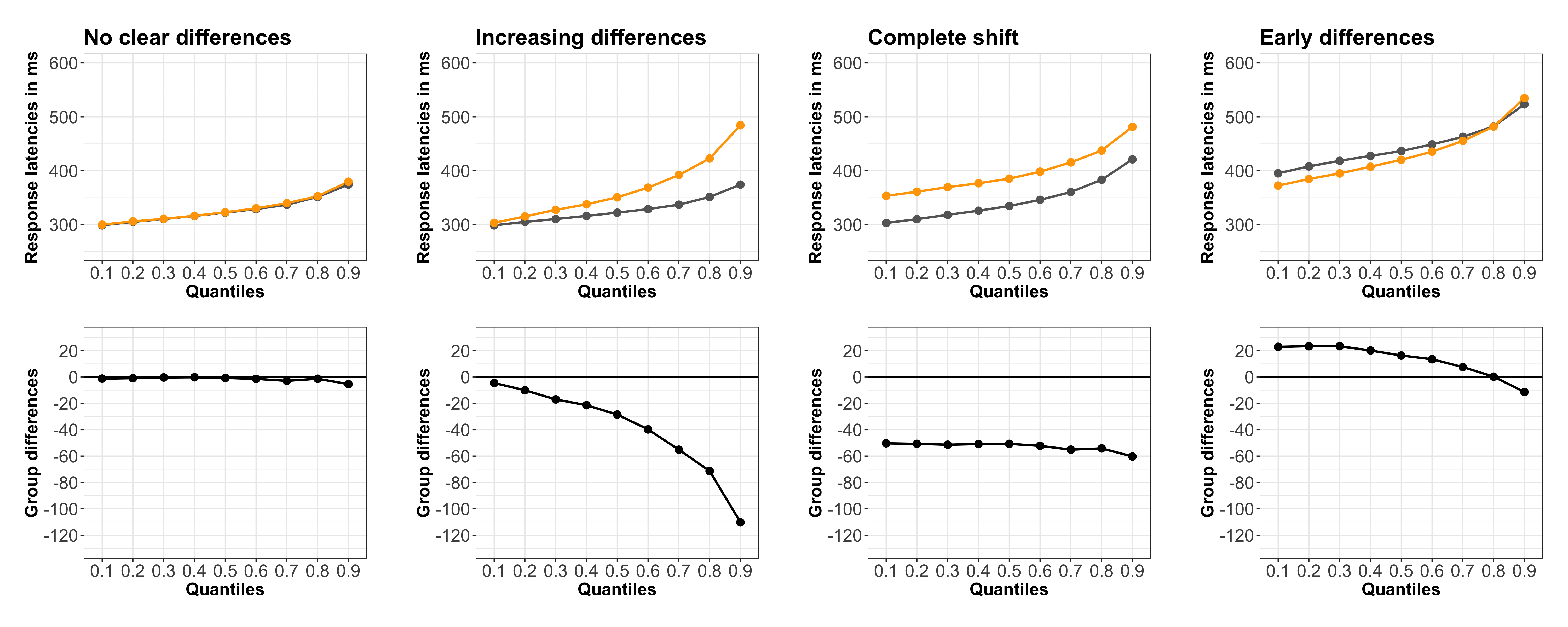{fig-align="center"}](https://garstats.wordpress.com/tag/vincentile/)## Set-upBelow are the packages you should install to ensure this document runs properly.```{r}#load packageslibrary(plyr)library(easystats)library(tidyverse)library(knitr)library(cowplot)library(ggeffects)library(here)library(data.table)library(ggrepel)library(brms)library(ggdist)library(emmeans)library(tidylog)library(tidybayes)library(hypr)library(cowplot)library(tidyverse)library(colorspace)library(ragg)library(cowplot)library(ggtext)library(MetBrewer)library(ggdist)library(modelbased)library(flextable)library(cmdstanr)library(brms)library(easystats)library(gt)process_ER_column <-function(x) {# Check if ER column value is numeric, if not, replace with Inf x <-ifelse(is.numeric(x), x, Inf)return(x)}```## Figure Theme```{r prep, message=FALSE}bold <-element_text(face ="bold", color ="black", size =16) #axis boldtheme_set(theme_minimal(base_size =15, base_family ="Arial"))theme_update(panel.grid.major =element_line(color ="grey92", size = .4),panel.grid.minor =element_blank(),axis.title.x =element_text(color ="grey30", margin =margin(t =7)),axis.title.y =element_text(color ="grey30", margin =margin(r =7)),axis.text =element_text(color ="grey50"),axis.ticks =element_line(color ="grey92", size = .4),axis.ticks.length =unit(.6, "lines"),legend.position ="top",plot.title =element_text(hjust =0, color ="black", family ="Arial",size =21, margin =margin(t =10, b =35)),plot.subtitle =element_text(hjust =0, face ="bold", color ="grey30",family ="Arial", size =14, margin =margin(0, 0, 25, 0)),plot.title.position ="plot",plot.caption =element_text(color ="grey50", size =10, hjust =1,family ="Arial", lineheight =1.05, margin =margin(30, 0, 0, 0)),plot.caption.position ="plot", plot.margin =margin(rep(20, 4)))pal <-c(met.brewer("Veronese", 3))``````{r}## flat violinplots### It relies largely on code previously written by David Robinson ### (https://gist.github.com/dgrtwo/eb7750e74997891d7c20) and ggplot2 by H Wickham#check if required packages are installed#Load packages# Defining the geom_flat_violin function. Note: the below code modifies the # existing github page by removing a parenthesis in line 50geom_flat_violin <-function(mapping =NULL, data =NULL, stat ="ydensity",position ="dodge", trim =TRUE, scale ="area",show.legend =NA, inherit.aes =TRUE, ...) {layer(data = data,mapping = mapping,stat = stat,geom = GeomFlatViolin,position = position,show.legend = show.legend,inherit.aes = inherit.aes,params =list(trim = trim,scale = scale, ... ) )}# horizontal nudge position adjustment# copied from https://github.com/tidyverse/ggplot2/issues/2733position_hnudge <-function(x =0) {ggproto(NULL, PositionHNudge, x = x)}PositionHNudge <-ggproto("PositionHNudge", Position,x =0,required_aes ="x",setup_params =function(self, data) {list(x = self$x) },compute_layer =function(data, params, panel) {transform_position(data, function(x) x + params$x) })``````{r}#| message: false#| cache: falsetheme_set(theme_linedraw() +theme(panel.grid =element_blank()))bayesplot::color_scheme_set(scheme ="brewer-Spectral")options(digits =3)```# Method: Experiment 1The preregistered analysis plan can be found here: https://osf.io/q3fjn. All raw and summary data, materials, and R scripts for pre-processing, analysis, and plotting for Experiments 1 can be found at https://osf.io/6sy7k/.## ParticipantsWe preregistered a sample size of 216. All participants were recruited through the university subject pool (SONA). A design with a sample size of 216 can detect effect sizes of δ≥ 0.2 with a probability of at least 0.90, assuming a one-sided criterion for detection that allows for a maximum Type I error rate of α=0.05. Per our exclusion criteria, we retained participants that were native English speakers, were over the age of 17, had overall accuracy on the LDT greater than 80%, and did not complete the experiment more than once. Due to our exclusion criteria, we oversampled participants. Because of this we randomly chose 36 participants from each list to reach our target sample size.## Apparatus and stimuliThe experiment was run using PsychoPy software and hosted on Pavlovia (www.pavlovia.org). You can see an example of the experiment by navigating to this website: <https://run.pavlovia.org/Jgeller112/ldt_dd_l1_jol_context>.We used 84 words and 84 nonwords for the LDT. Words were obtained from the the LexOPS package in R [@taylor2020a]. All of our words were matched on a number of different lexical dimensions. All words were nouns, 4-6 letters in length, had a known proportion of between 90%-100%, had a low neighborhood density (OLD20 score between 1-2), high concreteness, imageability, and word frequency. Our nonwords were were created using the English Lexicon Project [@balota2007]. Stimuli can be found at our OSF project page cited above.### BlurringBlurred stimuli were processed through the imager package in R [@imager] and a personal script (https://osf.io/gr5qv). Each image was processed through a high blur filter (Gaussian blur of 15) and low blur filter (Gaussian blur of 10). These pictures were then imported into PsychoPy as picture files. See Figure 2 for examples of what a clear, low blurred, and high blurred word would look like to the participant.{fig-align="center"}{fig-align="center"}{fig-align="center"}## DesignWe created two lists: One list (84 words; 28 clear, 28 low blur, 28 high blur) served as a study (old) list for the LDT task while the other list served as a test (new) list (84 words; 28 clear, 28, LB, 28, HB) for our recognition memory test that occurred after the LDT. We counterbalanced each list so each word served as an old word and a new world and were presented in clear, low blurred, and high blurred across participants. This resulted in six counterbalanced lists. Lists were assigned to participants so that across participants each word occurs equally often in the six possible conditions: clear old, LB old, HB old, clear new, LB new, and HB new. For the LDT task, we generated a set of 84 legal nonwords that we obtained from the English Lexicon Project. These 84 nonwords were used across all 6 lists.## ProcedureThe experiment consisted of two phases: an encoding phase (LDT) and a test phase. During the encoding phase, a fixation cross appeared at the center of the screen for 500 ms. The fixation cross was immediately replaced by a letter string in the same location. To continue to the next trial, participants had to decide if the letter string presented on screen was a word or not by either pressing designated keys on the keyboard ("m" or "z") or by tapping on designated areas on the screen (word vs. nonword) if they were using a cell phone/tablet. After the encoding phase, participants were given a surprise old/new recognition memory test. During the test phase, a word appeared in the center of the screen that either had been presented during study ("old") or had not been presented during study ("new"). Old words occurred in their original typeface, and following the counterbalancing procedure, each of the new words was presented as clear, low blurred, or high blurred. All words were individually randomized for each participant during both the study and test phases and progress was self-paced. After the experiment, participants were debriefed. The entire experiment lasted approximately 15 minutes.## Analysis PlanAll models were fit using The Stan modeling language [@grant2017] with the `brms`[@brms] package in in R . We only analyzed trials where the target stimulus was a word (Experiment 1a and 1b) or non-animal (Experiment 2). For the DDM, we excluded trials with RTs lower than 200 ms or higher than 2500 ms. For the accuracy analysis, we only excluded trials with RTs lower than 200 ms or higher than 2500 ms (% of trials). For Experiments 1a and 1b, we fit a model with blurring (clear vs. high blur vs. low blur). For Experiment 2, we fit a model with blurring and word frequency. The models included maximal random-effect structures justified by the design (Barr et al., 2013). This included random intercepts for participants and items, and a random slope by blurring level for each varying random intercept. Contrast codes for each variable were created using the `hypr` package in R [@hypr]. We fit the models twice: Once with contrast codes for high blur vs. clear and for high blur vs. Low blur and once with the low blur vs. clear contrast.In all experiments reported here, the statistical model was run with four chains of 5,000 Markov chain Monte Carlo iterations, with 1,000-iteration warmups for 4 chains (16,000 samples in total). [^expt1a-1]Convergence and stability of the Bayesian sampling is quantified by the Rˆ(R hat) diagnostics below 1.01 and Effective Sample SIze (ESS) greater than 1000 [@brms]. For both the RT data and accuracy data, we report our models with with weakly-informative priors for the population-level parameters. Using a weakly-informative prior as opposed to a default (which is an uniform prior where all effects are equally likely) allows for the calculation of evidence ratio (Bayes Factor) for one-sides tests. For the ex-Gaussian analysis we used a weak prior (i.e., N \~ (0, 100)). For the population-level effects in the accuracy and signal detection analyses, we used a Cauchy distribution with the mean of 0 and scale of 0.35 (cauchy \~ 0, 0.35)) recommended by [@kinoshita2023] for logistic regression.[^expt1a-1]: For the DDM we fit a model with 2,000 chains .For the marginal means and differences , we report the expected values under the posterior distribution and their 90% credible intervals (Cr. I.). For marginal mean differences, we also report the posterior probability that a difference δ is not zero. If a hypothesis states that δ \\\> 0, then it would be considered strong evidence for this hypothesis would be if zero is not included in the 90% Cr. I. of δ and the posterior P(δ \\\> 0) is close to one (by a reasonably clear margin). To extract the estimated marginal means from the posterior distribution of the fitted models we used a combination of `emmeans` R package [@emmeans-2]`bayestestr`[@bayestestR], and `brms`[@brms-2].Model quality was thoroughly assessed via predictive prior and posterior checks, Rhat and divergence diagnostics. In order to assess the evidence in favor or against our hypotheses, we used Evidence Ratio (ER, a generalization of Bayes factors allowing for directional hypotheses). An ER above 3 indicates moderate to substantial evidence for our hypothesis, below 0.3 indicates moderate to substantial evidence for the null hypothesis, and anything in between is inconclusive evidence [@BayesFactor].### Ex-GaussianFor the ex-Gaussian analyses we excluded trials with RTs lower than 200 ms or higher than 2500 ms as well as incorrect responses (% of trials).We used the ex-Gaussian distribution to model response times, with both the mean of the Gaussian component 𝜇 and the scale parameter ($$\sigma$$) of the exponential component 𝛽 (equaling the inverse of the rate parameter 𝜆) being allowed to vary between conditions. In addition, to better visualize the distributional features of the latency data, we computed the delta plots for all variables.Lastly, to model response accuracy, we used the Bernoulli distribution with a logit link. We only excluded trials with RTs lower than 200 ms or higher than 2500 ms (% of trials).### Diffusion ModelWe used a hierarchical-Bayesian variant of the Wiener diffusion model [@vandekerckhove2011] with accuracy coding. This model accounts for the entire data (i.e., RT distributions of correct and error trials) with three latent parameters: (a) the drift rate, a measure of the efficiency of information processing in the decision process, (b) the boundary separation, a measure of response caution that controls the speed-accuracy trade-off (this was fixed to .5), and (c) the non-decision time on-coding parametrization -- to each dataset.For the DDM, we excluded trials with RTs lower than 200 ms or higher than 2500 ms.### Recognition memoryFor our recognition memory data, we fit a Bayesian generalized linear multilevel model with a Bernoulli distribution with a probit link. In its simplest from, SDT models are regressions with a probit link. To estimate the SDT parameter of interest (\$d\^\$), we fit a Bayesian hierarchical generalized linear model with a binomial distribution probit link function to participant responses (their actual response (old vs. new)) as a function of actual item status (old vs. new) and blurring level. Traditional SDT analyses have proven to be an informative and efficient approach to analyzing binary accuracy data. However, considering the deficiency in precision and power in traditional analyses compared to mixed effects analyses, it is worth considering a Bayesian generalized linear mixed effect approach to SDT (see [@zloteanu2023] for a nice tutorial on Bayesian SDT models).# ResultsAll models presented no divergences, and all chains mixed well and produced comparable estimates (Rhat \< 1.01).## Accuracy```{r}#The data file is cleaned (participants >=.8, no duplicate participants, no participants < 17. )# get data from osfblur_acc <-read_csv("https://osf.io/xv5bd/download") %>% dplyr::filter(lex=="m")blur_acc_new<- blur_acc %>% dplyr::filter(rt >= .2& rt <=2.5)head(blur_acc)# get trials and how many elminated dim(blur_acc)dim(blur_acc_new)```The analysis of accuracy is is based on `r dim(blur_acc)[1]` data points. After removing fast and slow RTs we were left with `r dim(blur_acc_new)[1]` data point points (`r 1-dim(blur_acc_new)[1]/dim(blur_acc)[1]` %)## Contrast Code```{r}## Contrasts#hypothesisblurC <-hypr(HB~C, HB~LB, levels=c("C", "HB", "LB"))blurC#set contrasts in df blur_acc_new$blur <-as.factor(blur_acc_new$blur)contrasts(blur_acc_new$blur) <-contr.hypothesis(blurC)```## BRMs: Accuracy Model```{r}#| eval: false#| #weak priorprior_exp1 <-c(set_prior("cauchy(0,.35)", class ="b"))#fit modelfit_acc_weak <-brm(corr ~ blur + (1+blur|participant) + (1+blur|string), data=blur_acc_new, warmup =1000,iter =5000,chains =4, init=0, family =bernoulli(),cores =4,prior = prior_exp1, control =list(adapt_delta =0.9), backend="cmdstanr", save_pars =save_pars(all=T),sample_prior = T, threads =threading(4), file="fit_acc_context")```## Contrast Code```{r}## Contrasts#hypothesisblurC <-hypr(LB~C, levels=c("C", "HB", "LB"))blurC#set contrasts in df blur_acc_new$blur <-as.factor(blur_acc_new$blur)contrasts(blur_acc_new$blur) <-contr.hypothesis(blurC)```## BRMs: Accuracy Model```{r}#| eval: false#| #weak priorprior_exp1 <-c(set_prior("cauchy(0,.35)", class ="b"))#fit modelfit_acc_weak_lb <-brm(corr ~ blur + (1+blur|participant) + (1+blur|string), data=blur_acc_new, warmup =1000,iter =5000,chains =4, init=0, family =bernoulli(),cores =4,prior = prior_exp1, control =list(adapt_delta =0.9), backend="cmdstanr", save_pars =save_pars(all=T),sample_prior = T, threads =threading(4), file="fit_acc_context_lbc")``````{r}# get file from osfacc_c<-read_rds("https://osf.io/xwdzn/download")# get lowblur-c comparisonacc_lb <-read_rds("https://osf.io/wt3ry/download")```## Model SummaryUsing \`brms::hypothesis to extract support for each comparison of interest.```{r}acc_means <-emmeans(acc_c, specs="blur", type="response") %>%as.data.frame()``````{r}a <-hypothesis(acc_c, "blur1 < 0")b <-hypothesis(acc_c, "blur2 < 0")c<-hypothesis(acc_lb, "blur1 = 0")tab <-bind_rows(a$hypothesis, b$hypothesis, c$hypothesis) %>%mutate(Evid.Ratio=as.numeric(Evid.Ratio))%>%select(-Star)tab[, -1] <-t(apply(tab[, -1], 1, round, digits =3))tab %>%mutate(Hypothesis =c("High Blur - Clear < 0", "High Blur - Low Blur < 0", "Low Blur - Clear = 0 ")) %>%gt(caption=md("Table: Accuracy Directional Hypotheses Experiment 1")) %>%cols_align(columns=-1,align="right" )```### Accuracy SummaryClear words were better identified ($M$ = .985) compared to high blur words ($M$ = .962), b = `r a$hypothesis$Estimate`, 90% Cr.I\[`r a$hypothesis$CI.Lower`, `r a$hypothesis$CI.Upper`\], ER = `r process_ER_column(a$hypothesis$Evid.Ratio)`. Low blurred words were better identified ($M$ = .986) than high blurred words, $b$ = `r b$hypothesis$Estimate`, 90% Cr.I\[`r b$hypothesis$CI.Lower`, `r b$hypothesis$CI.Upper`\], ER = `r process_ER_column(b$hypothesis$Evid.Ratio)`. However, the evidence was weak for there being no significant difference in the identification accuracy between clear and low blurred words, $b$ = `r c$hypothesis$Estimate`, 90% Cr.I\[`r c$hypothesis$CI.Lower`, `r c$hypothesis$CI.Upper`\], ER = `r process_ER_column(c$hypothesis$Evid.Ratio)`.### Figures```{r}#| fig-cap: "Experiment 1: Accuracy"top_mean <-blur_acc %>%#get means for each blur cond for plot dplyr::filter(lex=="m")%>%group_by(blur)%>% dplyr::summarise(mean1=mean(corr)) %>% dplyr::ungroup()p_mean <-blur_acc %>%#get means participant x cond for plottin dplyr::filter(lex=="m")%>% dplyr::group_by(participant, blur)%>% dplyr::summarise(mean1=mean(corr))p3 <-ggplot(p_mean, aes(x = blur , y = mean1, fill = blur)) +coord_cartesian(ylim =c(.5,1)) + ggdist::stat_halfeye(aes(y = mean1,color = blur,fill =after_scale(lighten(color, .5)) ),shape =18,point_size =3,interval_size =1.8,adjust = .5,.width =c(0, 1) ) +geom_point(aes(x = blur, y = mean1, colour = blur),position =position_jitter(width = .05), size =1, shape =20)+geom_boxplot(aes(x = blur, y = mean1, fill = blur),outlier.shape =NA, alpha = .5, width = .1, colour ="black")+labs(subtitle ="Word Accuracy: Context Reinstatement")+scale_color_manual(values=met.brewer("Cassatt2", 3))+scale_fill_manual(values=met.brewer("Cassatt2", 3))+stat_summary(fun=mean, geom="point", colour="darkred", size=3)+labs(y ="Accuracy", x ="Blur") +geom_label_repel(data=top_mean, aes(y=mean1, label=round(mean1, 2)), color="black", min.segment.length =0, seed =42, box.padding =0.5) +theme(axis.text=bold) +theme(legend.position ="none")# ggsave('place.png', width = 8, height = 6)p3```## RTs## BRMs: RTs```{r}#load data from osfrts <-read_csv("https://osf.io/xv5bd/download")``````{r}blur_rt<- rts %>%group_by(participant) %>% dplyr::filter(corr==1, lex=="m")#only include nonwordsblur_rt_new <- blur_rt %>% dplyr::filter(rt >= .2& rt <=2.5)%>%mutate(rt_ms=rt*1000)dim(blur_rt)dim(blur_rt_new)```The analysis of RTs (correct trials and words) is based on `r dim(blur_rt_new)[1]` data points, after removing fast and slow RTs (`r 1-dim(blur_rt_new)[1]/dim(blur_rt)[1]` %)### Density Plots```{r}p <-ggplot(blur_rt_new, aes(rt_ms, group = blur, fill = blur)) +geom_density(colour ="black", size =0.75, alpha =0.5) +scale_fill_manual(values=c("grey40", "orange1", "red")) +theme(axis.title =element_text(size =16, face ="bold", colour ="black"), axis.text =element_text(size =16, colour ="black"), plot.title =element_text(face ="bold", size =20)) +coord_cartesian(xlim=c(600, 1100)) +scale_x_continuous(breaks=seq(600,1100,100)) +labs(title ="Density Plot By Blur", y ="Density", x ="Response latencies in ms") +theme_bw() p``````{r}## Contrasts#hypothesisblurC <-hypr(HB~C, HB~LB, levels=c("C", "HB", "LB"))blurC#set contrasts in df blur_rt$blur <-as.factor(blur_rt$blur)contrasts(blur_rt$blur) <-contr.hypothesis(blurC)```### Ex-Gaussian#### Model Set-up```{r, eval=FALSE}library(cmdstanr)bform_exg1 <-bf(rt ~0+ blur + (1+ blur |p| participant) + (1+ blur|i| string),sigma ~0+ blur + (1+ blur |p|participant) + (1+ blur |i| string),beta ~0+ blur + (1+ blur |p|participant) + (1+ blur |i| string))```#### Run Model```{r, eval=FALSE}#| eval: false#| prior_exp1 <-c(set_prior("normal(0,100)", class ="b", coef=""))fit_exg1 <-brm(bform_exg1, data = blur_rt,warmup =1000,iter =5000,chains =4,prior = prior_exp1,family =exgaussian(),init =0,cores =4, sample_prior = T, save_pars =save_pars(all=T),control =list(adapt_delta =0.8), backend="cmdstanr", threads =threading(4))setwd(here::here("Context", "RT_BRM_Model"))save(fit_exg1, file ="blmm_rt_context_05-25-23.RData")``````{r}#load rdata for model #load_github_data("https://osf.io/uxc2f/download")#setwd(here::here("Expt1", "BRM_ACC_RT"))#here::here("Expt1", "BRM_ACC_RT", #"blmm_rt_context_05-25-23.RData"))# no intercept model - easier to fit priors on all levels of factor fit_c <-read_rds("https://osf.io/82nre/download")```## Model summary### Hypotheses```{r}a <-hypothesis(fit_c, "blurHB - blurC > 0", dpar="mu")b <-hypothesis(fit_c, "blurHB - blurLB > 0", dpar="mu")c <-hypothesis(fit_c, "blurLB - blurC > 0", dpar="mu")d <-hypothesis(fit_c, "sigma_blurHB - sigma_blurC > 0", dpar="sigma")e <-hypothesis(fit_c, "sigma_blurHB - sigma_blurLB > 0", dpar="sigma")f <-hypothesis(fit_c, "sigma_blurLB - sigma_blurC = 0", dpar="sigma")g <-hypothesis(fit_c, "beta_blurHB - beta_blurC > 0", dpar="beta")h <-hypothesis(fit_c, "beta_blurHB - beta_blurLB > 0", dpar="beta")i <-hypothesis(fit_c, "beta_blurLB - beta_blurC = 0", dpar="c")tab <-bind_rows(a$hypothesis, b$hypothesis, c$hypothesis, d$hypothesis, e$hypothesis, f$hypothesis, g$hypothesis, h$hypothesis, i$hypothesis) %>%mutate(Evid.Ratio=as.numeric(Evid.Ratio))%>%select(-Star)tab[, -1] <-t(apply(tab[, -1], 1, round, digits =3))tab %>%mutate(parameter=c("mu","mu", "mu", "sigma", "sigma", "sigma", "beta", "beta", "beta"))%>%mutate(Hypothesis =c("High Blur - Clear > 0", "High Blur - Low Blur > 0", "Low Blur - Clear > 0 ", "High Blur - Clear > 0", "High Blur - Low Blur > 0", "Low Blur - Clear = 0","High Blur - Clear > 0", "High Blur - Low Blur > 0", "Low Blur - Clear = 0 "))%>%gt(caption=md("Table: Ex-Gaussian Model Results Experiment 1")) %>%cols_align(columns=-1,align="right" )```### Ex-Gaussian plots```{r}library(patchwork)p1<-conditional_effects(fit_c, "blur", dpar ="mu")p2<-conditional_effects(fit_c, "blur", dpar ="sigma")p3<-conditional_effects(fit_c, "blur", dpar ="beta")p1 <-plot(p1, plot =FALSE)[[1]] +labs(x ="Blur", y ="Mu", color ="blur", fill ="blur") +scale_x_discrete(labels=c('Clear', 'High Blur', 'Low Blur')) +theme_minimal(base_size=20)p2 <-plot(p2, plot =FALSE)[[1]] +labs(x ="Blur", y ="Sigma", color ="blur", fill ="blur") +scale_x_discrete(labels=c('Clear', 'High Blur', 'Low Blur')) +theme_minimal(base_size=20)p3 <-plot(p3, plot =FALSE)[[1]] +labs(x ="Blur", y ="Beta/Tau", color ="blur", fill ="blur") +scale_x_discrete(labels=c('Clear', 'High Blur', 'Low Blur')) +theme_minimal(base_size=20)p_all = p1+p2+p3p_allggsave("p_all-ex.png", width=8, height=4, dpi=500)```#### Write-up##### Ex-GaussianA visualization of how blurring affected processing during word recognition can be seen Figure. 3. Beginning with the μ parameter, there was greater shifting for high blurred words compared to clear words, *b* = `r a$hypothesis$Estimate`, 90% Cr.I\[`r a$hypothesis$CI.Lower`, `r a$hypothesis$CI.Upper`\], ER = `r process_ER_column(a$hypothesis$Evid.Ratio)`, and low blur words, b = `r b$hypothesis$Estimate`, 90% Cr.I\[`r b$hypothesis$CI.Lower`, `r b$hypothesis$CI.Upper`\], ER = `r process_ER_column(b$hypothesis$Evid.Ratio)`. Analyses of the σ and τ parameters yielded a similar pattern. Variance was higher for high blurred words compared to clear words, *b* = `r d$hypothesis$Estimate`, 90% Cr.I\[`r d$hypothesis$CI.Lower`, `r d$hypothesis$CI.Upper`\], ER = `r process_ER_column(d$hypothesis$Evid.Ratio)`, and low blurred words, *b* = `r e$hypothesis$Estimate`, 90% Cr.I\[`r e$hypothesis$CI.Lower`, `r e$hypothesis$CI.Upper`\], ER = `r process_ER_column(e$hypothesis$Evid.Ratio)`. Finally, there was greater skewing for high blurred words compared to clear words , b = `r g$hypothesis$Estimate`, 90% Cr.I\[`r g$hypothesis$CI.Lower`, `r g$hypothesis$CI.Upper`\], ER = `r g$hypothesis$Evid.Ratio` and low blurred words, b = `r h$hypothesis$Estimate`, 90% Cr.I\[`r h$hypothesis$CI.Lower`, `r h$hypothesis$CI.Upper`\], ER = `r h$hypothesis$Evid.Ratio`. Low blurred words compared to clear words only differed on the μ parameter, $b$ = `r c$hypothesis$Estimate`, 90% Cr.I\[`r c$hypothesis$CI.Lower`, `r c$hypothesis$CI.Upper`\], ER = `r process_ER_column(c$hypothesis$Evid.Ratio)`, with greater shifting for low blurred words. For $\tau$ and $\sigma$, the 95 Cr.I crossed zero and the ER was greater than 100.## Diffusion model```{r}blur_rt_diff<- rts %>%group_by(participant) %>% dplyr::filter(rt >= .2& rt <=2.5)%>% dplyr::filter(lex=="m")head(blur_rt_diff)``````{r}#| eval: falseformula <-bf(rt |dec(corr) ~0+ blur + (1+ blur|p|participant) + (1+blur|i|string), ndt ~0+ blur + (1+ blur|p|participant) + (1+blur|i|string),bias =.5)bprior <-prior(normal(0, 1), class = b) +prior(normal(0, 1), class = b, dpar = ndt)+prior(normal(0, 1), class = sd) +prior(normal(0, 1), class = sd, dpar = ndt) +prior("normal(0, 0.3)", class ="sd", group ="participant")+prior("normal(0, 0.3)", class ="sd", group ="string")``````{r}#| eval: false#| make_stancode(formula, family =wiener(link_bs ="identity", link_ndt ="identity",link_bias ="identity"),data = blur_rt_diff, prior = bprior)tmp_dat <-make_standata(formula, family =wiener(link_bs ="identity", link_ndt ="identity",link_bias ="identity"),data = blur_rt_diff, prior = bprior)str(tmp_dat, 1, give.attr =FALSE)initfun <-function() {list(b =rnorm(tmp_dat$K),bs=.5, b_ndt =runif(tmp_dat$K_ndt, 0.1, 0.15),sd_1 =runif(tmp_dat$M_1, 0.5, 1),sd_2 =runif(tmp_dat$M_2, 0.5, 1),z_1 =matrix(rnorm(tmp_dat$M_1*tmp_dat$N_1, 0, 0.01), tmp_dat$M_1, tmp_dat$N_1),z_2 =matrix(rnorm(tmp_dat$M_2*tmp_dat$N_2, 0, 0.01), tmp_dat$M_2, tmp_dat$N_2),L_1 =diag(tmp_dat$M_1),L_2 =diag(tmp_dat$M_2) )}``````{r}#| eval: falsefit_wiener1 <-brm(formula, data = blur_rt_diff,family =wiener(link_bs ="identity", link_ndt ="identity",link_bias ="identity"),prior = bprior, init=initfun,iter =2000, warmup =500, chains =4, cores =4,file="weiner_diff_1", backend ="cmdstanr", threads =threading(4), control =list(max_treedepth =15))``````{r}#diff object on osffit_wiener <-read_rds("https://osf.io/hqauz/download")```### Diffusion Hypotheses```{r}a <-hypothesis(fit_wiener, "blurHB - blurC < 0", dpar="mu")b <-hypothesis(fit_wiener, "blurHB - blurLB < 0", dpar="mu")c =hypothesis(fit_wiener, "blurLB - blurC = 0", dpar="mu")d <-hypothesis(fit_wiener, "ndt_blurHB - ndt_blurC > 0", dpar="ndt")e <-hypothesis(fit_wiener, "ndt_blurHB - ndt_blurLB > 0", dpar="ndt")f <-hypothesis(fit_wiener, "ndt_blurLB - ndt_blurC > 0", dpar="ndt")tab <-bind_rows(a$hypothesis, b$hypothesis, c$hypothesis, d$hypothesis, e$hypothesis, f$hypothesis) %>%mutate(Evid.Ratio=as.numeric(Evid.Ratio))%>%select(-Star)tab[, -1] <-t(apply(tab[, -1], 1, round, digits =3))tab %>%mutate(parameter=c("v","v", "v", "T_er", "T_er", "T_er")) %>%mutate(Hypothesis =c("High Blur - Clear > 0", "High Blur - Low Blur > 0", "Low Blur - Clear = 0 ", "High Blur - Clear > 0", "High Blur - Low Blur > 0", "Low Blur - Clear = 0"))%>%gt(caption=md("Table: Diffusion Model Results for Experiment 1")) %>%cols_align(columns=-1,align="right" )``````{r}me_mu <-conditional_effects(fit_wiener, "blur", dpar ="mu") me_mu_plot <-plot(me_mu, plot =FALSE)[[1]] +labs(x ="Blur", y ="Drift Rate", color ="blur", fill ="blur") +scale_x_discrete(labels=c('Clear', 'High Blur', 'Low Blur')) +theme_minimal(base_size=20)me_mu_plot``````{r}me_ndt <-conditional_effects(fit_wiener, "blur", dpar ="ndt") me_ndt_plot <-plot(me_ndt, plot =FALSE)[[1]] +labs(x ="Blur", y ="Non-Decision Time", color ="blur", fill ="blur") +scale_x_discrete(labels=c('Clear', 'High Blur', 'Low Blur')) +theme_minimal(base_size=20)p_all_1 = p_all / (me_ndt_plot + me_mu_plot)p_all_1ggsave("p_all-diff.png", width=12, height=8, dpi=500)```### Write-up#### Diffusion ModelHigh blurred words had lower drift rate than clear words, b = `r a$hypothesis$Estimate`, 90% Cr.I\[`r a$hypothesis$CI.Lower`, `r a$hypothesis$CI.Upper`\], ER = `r process_ER_column(a$hypothesis$Evid.Ratio)`, and low blurred words, b = `r b$hypothesis$Estimate`, 90% Cr.I\[`r b$hypothesis$CI.Lower`, `r b$hypothesis$CI.Upper`\], ER = `r process_ER_column(b$hypothesis$Evid.Ratio)`. There was no difference in drift rate between low blurred words and cleared words, b = `r c$hypothesis$Estimate`, 90% Cr.I\[`r c$hypothesis$CI.Lower`, `r c$hypothesis$CI.Upper`\], ER = `r process_ER_column(c$hypothesis$Evid.Ratio)`. Non-decision time was higher for high blurred words compared to clear words, b = `r d$hypothesis$Estimate`, 90% Cr.I\[`r d$hypothesis$CI.Lower`, `r d$hypothesis$CI.Upper`\], ER = `r process_ER_column(d$hypothesis$Evid.Ratio)`, and low blurred words, b = `r e$hypothesis$Estimate`, 90% Cr.I\[`r e$hypothesis$CI.Lower`, `r e$hypothesis$CI.Upper`\], ER = `r process_ER_column(e$hypothesis$Evid.Ratio)`. Low blurred words had a higher non-decision time that clear words, b = `r f$hypothesis$Estimate`, 90% Cr.I\[`r f$hypothesis$CI.Lower`, `r f$hypothesis$CI.Upper`\], ER = `r process_ER_column(f$hypothesis$Evid.Ratio)`.## Quantile Plots/Vincentiles::: panel-tabset### Figure 1```{r}#Delta plots (one per subject) quibble <-function(x, q =seq(.1, .9, .2)) {tibble(x =quantile(x, q), q = q)}data.quantiles <- rts %>% dplyr::filter(rt >= .2| rt <=2.5) %>% dplyr::group_by(participant,blur,corr) %>% dplyr::filter(lex=="m")%>% dplyr::summarise(RT =list(quibble(rt, seq(.1, .9, .2)))) %>% tidyr::unnest(RT)data.delta <- data.quantiles %>% dplyr::filter(corr==1) %>% dplyr::select(-corr) %>% dplyr::group_by(participant, blur, q) %>% dplyr::summarize(RT=mean(x))``````{r}#Delta plots (based on vincentiles)vincentiles <- data.quantiles %>% dplyr::filter(corr==1) %>% dplyr::select(-corr) %>% dplyr::group_by(blur,q) %>% dplyr::summarize(RT=mean(x)) v=vincentiles %>% dplyr::group_by(blur,q) %>% dplyr::summarise(MRT=mean(RT))v <- v %>%mutate(blur=ifelse(blur=="HB", "High blur", ifelse(blur=="LB", "Low blur", "Clear")))v$blur<-factor(v$blur, level=c("High blur", "Low blur", "Clear"))p <-ggplot(v, aes(x = q, y = MRT*1000, colour = blur, group=blur))+geom_line(size =1) +geom_point(size =3) +scale_colour_manual(values=met.brewer("Cassatt2", 3)) +scale_y_continuous(breaks=seq(500,1600,100)) +theme(legend.title=element_blank())+coord_cartesian(ylim =c(500, 1600)) +scale_x_continuous(breaks=seq(.1,.9, .2))+geom_label_repel(data=v, aes(x=q, y=MRT*1000, label=round(MRT*1000,0)), color="black", min.segment.length =0, seed =42, box.padding =0.5, size=10) +labs(title ="Quantile Analysis", x ="Quantiles", y ="Response latencies in ms") +theme_minimal(base_size=36) p```### Figure 2```{r}p2 <-ggplot(data=v,aes(y=MRT, x=fct_relevel(blur, c("HB", "C", "LB")), color=q)) +geom_line()+geom_point(size=4) +labs(x="Blur") +scale_x_discrete(labels=c('High Blur', 'Low Blur', 'Clear'))p2```## :::### Delta Plots#### Clear vs. High Blur```{r}#| fig-cap: "Delta plots depicting the magnitude of the effect over time in Experiment 1. Each dot represents the mean RT at the .1, .3, .5, .7 and .9 quantiles."#| v_chb <- v %>% dplyr::filter(blur=="Clear"| blur=="High blur") %>% dplyr::group_by(q)%>%mutate(mean_rt =mean(MRT)*1000) %>%ungroup() %>%select(-q) %>% tidyr::pivot_wider(names_from ="blur", values_from ="MRT") %>%mutate(diff=`High blur`*1000-Clear*1000)p1 <-ggplot(v_chb, aes(x = mean_rt, y = diff)) +geom_abline(intercept =0, slope =0) +geom_line(size =1, colour ="black") +geom_point(size =3, colour ="black") +theme(legend.position ="none") +theme_minimal(base_size=36)+scale_y_continuous(breaks=seq(110,440,50)) +coord_cartesian(ylim =c(110, 440)) +scale_x_continuous(breaks=seq(600,1300, 200))+geom_label_repel(data=v_chb, aes(y=diff, label=round(diff,0)), color="black", min.segment.length =0, seed =42, box.padding =0.5, size=10)+labs( title ="Delta Plots: Clear - High Blur", x ="Mean RT per quantile", y ="Group differences") p1```#### Clear vs. Low Blur```{r}#| fig-cap: "Delta plots depicting the magnitude of the effect over time in Experiment 1. Each dot represents the mean RT at the .1, .3, .5, .7 and .9 quantiles." v_clb <- v %>% dplyr::filter(blur=="Clear"| blur=="Low blur") %>% dplyr::group_by(q)%>%mutate(mean_rt =mean(MRT)*1000) %>%ungroup() %>%select(-q) %>% tidyr::pivot_wider(names_from ="blur", values_from ="MRT") %>%mutate(diff=`Low blur`*1000-Clear*1000)p2 <-ggplot(v_clb, aes(x = mean_rt, y = diff)) +geom_abline(intercept =0, slope =0) +geom_line(size =1, colour ="black") +geom_point(size =3, colour ="black") +theme_minimal(base_size=36) +theme(legend.position ="none") +scale_y_continuous(breaks=seq(-10, 70, 10)) +coord_cartesian(ylim =c(-10, 70)) +scale_x_continuous(breaks=seq(500,1150, 200))+geom_label_repel(data=v_clb, aes(y=diff, label=round(diff,0)), color="black", min.segment.length =0, seed =42, box.padding =0.5, size=10) +labs( title ="Delta Plots: Low Blur - Clear", x ="Mean RT per quantile", y ="Group differences")p2```#### High Blur vs. Low Blur```{r}#| fig-cap: "Delta plots depicting the magnitude of the effect over time in Experiment 1. Each dot represents the mean RT at the .1, .3, .5, .7 and .9 quantiles."v_hlb <- v %>% dplyr::filter(blur=="High blur"| blur=="Low blur") %>% dplyr::group_by(q)%>%mutate(mean_rt =mean(MRT)*1000) %>%ungroup() %>%select(-q) %>% tidyr::pivot_wider(names_from ="blur", values_from ="MRT") %>%mutate(diff=`High blur`*1000-`Low blur`*1000)p3 <-ggplot(v_hlb, aes(x = mean_rt, y = diff)) +geom_abline(intercept =0, slope =0) +geom_line(size =1, colour ="black") +geom_point(size =3, colour ="black") +theme_minimal(base_size =36) +theme(legend.position ="none") +scale_x_continuous(breaks=seq(600,1350, 200))+geom_label_repel(data=v_hlb, aes(y=diff, label=round(diff,0)), color="black", min.segment.length =0, seed =42, box.padding =0.5, size=10)+labs( title ="Delta Plots High Blur - Low Blur", x ="Mean RT per quantile", y ="Group differences")p3``````{r}p / (p1 + p2 + p3)# save figureggsave(filename='./figures/figure_kde.png',width=12,height=8) ```## BRM: Conditionalized Memory- $D\prime$```{r}mem_c <-read_csv("https://osf.io/xjvc7/download")head(mem_c)```## Contrast code```{r}## Contrasts#hypothesisblurC <-hypr(HB~C, HB~LB, levels=c("C", "HB", "LB"))blurC#set contrasts in df mem_c$blur <-as.factor(mem_c$blur)contrasts(mem_c$blur) <-contr.hypothesis(blurC)```## BRM Model```{r}#| eval: false#| prior_exp2 <-c(set_prior("cauchy(0,.35)", class ="b"))fit_mem_c <-brm(sayold ~0+ isold*blur + (1+isold*blur|participant) + (1+isold*blur|string), data=mem_c, warmup =1000,iter =5000,chains =4, init=0, family =bernoulli(link ="probit"),cores =4, control =list(adapt_delta =0.9),prior=prior_exp2, sample_prior = T, file="blmm_sdt_c_nointercept"save_pars =save_pars(all=T),backend="cmdstanr",threads =threading(4))```### Marginal Means and Differences```{r}fit_mem1 <-read_rds("https://osf.io/xsvgt/download")sd_lb <-read_rds("https://osf.io/4qp38/download")```## Test Hypotheses### High Blur \> Clear```{r}#HB > Ca <-hypothesis(fit_mem1 , "isold1:blur1 > 0")b <-hypothesis(fit_mem1 , "isold1:blur2 > 0")c <-hypothesis(sd_lb , "isold1:blur1 = 0")tab <-bind_rows(a$hypothesis, b$hypothesis, c$hypothesis) %>%mutate(Evid.Ratio=as.numeric(Evid.Ratio))%>%select(-Star)tab[, -1] <-t(apply(tab[, -1], 1, round, digits =3))tab %>%gt(caption=md("Table: Memory Directional Hypotheses Experiment 1")) %>%cols_align(columns=-1,align="right" )```## Write-up### SensitivityHigh blur words were better remembered than clear words, $\beta$ = `r a$hypothesis$Estimate`, 90% Cr.I\[`r a$hypothesis$CI.Lower`, `r a$hypothesis$CI.Upper`\], ER = `r process_ER_column(a$hypothesis$Evid.Ratio)`, and low blurred words, $\beta$ = `r b$hypothesis$Estimate`, 90% Cr.I\[`r b$hypothesis$CI.Lower`, `r b$hypothesis$CI.Upper`\], ER = `r process_ER_column(b$hypothesis$Evid.Ratio)`. There was no difference in sensitivity between clear words and low blurred words, $\beta$ = `r c$hypothesis$Estimate`, 90% Cr.I\[`r c$hypothesis$CI.Lower`, `r c$hypothesis$CI.Upper`\], ER = `r process_ER_column(b$hypothesis$Evid.Ratio)`## Exploratory### Bias```{r}a <-hypothesis(fit_mem1 , "blur2 < 0")b <-hypothesis(sd_lb , "blur1 < 0")c<-hypothesis(fit_mem1 , "blur1= 0")```Low blurred words had a bias towards more "old" responses compared to clear words, \\$\beta$ = `r b$hypothesis$Estimate`, 90% Cr.I\[`r b$hypothesis$CI.Lower`, `r b$hypothesis$CI.Upper`\], ER = `r process_ER_column(b$hypothesis$Evid.Ratio)`, and high blurred words, $\beta$ = `r a$hypothesis$Estimate`, 90% Cr.I\[`r a$hypothesis$CI.Lower`, `r a$hypothesis$CI.Upper`\], ER = `r process_ER_column(a$hypothesis$Evid.Ratio)`. There was no difference in bias between high blurred words and clear words, $\beta$ = `r c$hypothesis$Estimate`, 90% Cr.I\[`r c$hypothesis$CI.Lower`, `r c$hypothesis$CI.Upper`\], ER = `r process_ER_column(c$hypothesis$Evid.Ratio)`.### D', C, and Differences```{r}# (Negative) criteriaemm_m1_c1 <-emmeans(fit_mem1, ~blur) %>% parameters::parameters(centrality ="mean")# Differences in (negative) criteriaemm_m1_c2 <-emmeans(fit_mem1, ~blur) %>%contrast("pairwise") %>% parameters::parameters(centrality ="mean")# Dprimes for three groupsemm_m1_d1 <-emmeans(fit_mem1, ~isold + blur) %>%contrast("revpairwise", by ="blur") %>% parameters::parameters(centrality ="mean")# Differences between groupsemm_m1_d2 <-emmeans(fit_mem1, ~isold + blur) %>%contrast(interaction =c("revpairwise", "pairwise")) %>% parameters::parameters(centrality ="mean")``````{r}#| fig-width: 12#| fig-height: 8#| fig-cap: Posterior distributions and 90%CIs of the criterion and dprime parameters, or differences therein, from the conditionalized modelemm_m1_c1 <-emmeans(fit_mem1, ~blur) emm_m1_c2 <-emmeans(fit_mem1, ~blur) %>%contrast("pairwise")# Dprimes for three groupsemm_m1_d1 <-emmeans(fit_mem1, ~isold + blur) %>%contrast("revpairwise", by ="blur")# Differences between groupsemm_m1_d2 <-emmeans(fit_mem1, ~isold + blur) %>%contrast(interaction =c("revpairwise", "pairwise")) tmp <-bind_rows(bind_rows(gather_emmeans_draws(emm_m1_d1) %>%group_by(blur) %>%select(-contrast),gather_emmeans_draws(emm_m1_d2) %>%rename(blur = blur_pairwise ) %>%group_by(blur) %>%select(-isold_revpairwise) ),bind_rows(gather_emmeans_draws(emm_m1_c1),gather_emmeans_draws(emm_m1_c2) %>%rename(blur = contrast ) ),.id ="Parameter") %>%mutate(Parameter =factor(Parameter, labels =c("d-prime", "Criterion"))) %>%mutate(t =if_else(str_detect(blur, " - "), "Differences", "Group means") %>%fct_inorder(),blur =fct_inorder(blur) )tmp %>%ungroup() %>%mutate(.value =if_else(Parameter =="Criterion", .value *-1, .value)) %>%mutate(Parameter =fct_rev(Parameter)) %>%mutate(blur=case_when( blur=="C"~"Clear", blur=="C - HB"~"Clear - High blur", blur=="HB"~"High blur", blur=="LB"~"Low blur", blur=="C - LB"~"Clear - Low blur", TRUE~"High blur - Low blur" )) %>%ggplot(aes(blur, .value)) +labs(x ="Blurring Level (or difference)",y ="Parameter value" ) +stat_halfeye(colour="green") +facet_grid(Parameter~t, scales ="free") +geom_hline(yintercept =0, linewidth = .25) +theme_minimal(base_size=25)ggsave("expt1a-dprime.png", width=19, height=8, dpi=300)``````{r}library(ggdist)#classic SDTsdt <- mem_c %>%dplyr::mutate(type ="hit",type =ifelse(isold==1& sayold==0, "miss", type),type =ifelse(isold==0& sayold==0, "cr", type), # Correct rejectiontype =ifelse(isold==0& sayold==1, "fa", type))sdt <- sdt %>%dplyr::group_by(participant, blur, type) %>%dplyr::summarise(count =n()) %>%tidyr::spread(type, count) # Format data to one row per personsdt2 <- sdt %>%dplyr::group_by(participant, blur)%>%dplyr::mutate(hr = hit / (hit+miss),fa = fa / (fa+cr)) %>%dplyr::mutate(hr=case_when(is.na(hr) ~0.99,TRUE~ hr),fa=case_when(is.na(fa) ~0.01,TRUE~ fa),zhr=qnorm(hr),zfa=qnorm(fa),dprime = zhr-zfa, crit =-0.5* (zhr + zfa))%>%ungroup()top_mean <- sdt2 %>%#get means for plot dplyr::group_by(blur)%>% dplyr::summarise(mean1=mean(dprime))p_mean <-sdt2 %>%#get means for plot dplyr::group_by(participant, blur)%>% dplyr::summarise(mean1=mean(dprime))```## DiscussionExperiment 1a successfully replicated the pattern of results found in @rosner2015. Specifically, we found high blurred words had lower accuracy than clear and low blurred words, but had better memory.Adding to this, we utilized cognitive and mathematical modeling to gain further insights into the mechanisms underlying the perceptual disfluency effect. Descriptively, high blurred words induced a more pronounced shift in the RT distribution (μ) and exhibited a higher degree of skew (τ) compared to clear and low blurred words. However, low blurred words did not differ compared to clear words on $\mu$ or $\beta$. These patterns can be clearly seen in our quantile delta plots in Fig. 3.We also fit the RTs and accuracy data to a diffusion model, which allowed us to make stronger inferences as it relates to stages of processing. High blurred words impacted both an early, non-decision, component evinced by higher $T_{er}$ and a later more analytic, component evinced by a lower $v$ than clear or low blurred words. On the other hand, low blurred words only affected $T_{er}$.We present evidence that different levels of disfluency can influence distinct stages of encoding, potentially contributing to the presence or absence of a mnemonic effect for perceptually blurred stimuli. Unlike most studies that commonly employ a single level of disfluency, our study incorporated two levels of disfluency. The results indicate that a subtle manipulation such as low blur primarily affects early processing stages, whereas a more pronounced perceptual manipulation (i.e., high blur) impacts both early and late processing stages. Regarding recognition memory, high blurred stimuli were better recognized compared to low blurred and clear words. This suggests that in order to observe a perceptual disfluency effect, the perceptual manipulation must be sufficiently disfluent to do so.Given the important theoretical implications of these findings, Experiment 1b served as a conceptual replication. Due to the bias observed in the recognition memory test (i.e., low blurred words were responded to more liberally), we will not present old and new items as blurred, instead all of the words will be presented in a clear, different, font at test.


